Is There Any Correlation Between Earnings Surprises and Stock Price Movements?

Use Python to pull earnings surprises and stock prices data to see if there is any correlation between the two

Many times when looking at the price movement of a stock after its earnings release, you may realize that earnings surprises (where the actual earnings is different from the estimates) can cause a stock to either gap up or down. Sometimes, albeit counterintuitively, a positive earnings surprise may cause a stock price to gap down instead.

Wouldn’t it be good to gather all the historical data of earnings surprises and stock price movements of your favorite stocks to do a quick correlation study? This is exactly what we will do in today’s article.

The full code of this project is given in the following repository on GitHub. Let’s get started!

Import Packages

First, we import the packages needed for data processing and plotting. We also need packages to deal with dates, as we will be scraping stock prices data of different dates to measure the stock price movement. We also need packages to parse different financial data, such as the stock prices and the earnings, from Financial Modelling Prep API before we put everything together. The data from Financial Modelling Prep API is in JSON format, which we will need to parse into a Python dictionary through the packages and function below.

# for data processing
import pandas as pd
import numpy as np

# for plotting
import matplotlib.pyplot as plt
plt.rcParams['figure.figsize'] = [12, 6]
import seaborn as sns
# for coloring heatmap later
from matplotlib.colors import LinearSegmentedColormap
from matplotlib.colors import TwoSlopeNorm 

# for dealing with dates
import datetime

# for dealing with environment variables
import os

# For parsing financial data (stock price and earnings) from financialmodelingprep api
from urllib.request import urlopen
import json
def get_jsonparsed_data(url):
    response = urlopen(url)
    data = response.read().decode("utf-8")
    return json.loads(data)

# Financialmodelingprep api url
base_url = "https://financialmodelingprep.com/api/v3/"

2. Set Up API Key for FMP Endpoint

The Financial Modeling Prep (FMP) API is an accurate financial data (i.e. stocks, earnings, historical data, market sentiment, financial statements etc.) API. You need to obtain the Financial Modeling Prep (FMP) API key (sign up here). There is also a free version where you can get 250 calls per day for free, which is enough to run the steps below. The paid version gives you a lot more benefits though.

Today, we are using it to obtain the

1. all historical earnings estimates and actual earnings results for stock tickers of interest
2. historical prices of stocks over a range of dates for stock tickers of interest

We will learn to scrap both the data above from the API and perform some analysis on them.

2.1. FMP API Key and Endpoint

Next we define the base URL endpoint for the FMP API “https://financialmodelingprep.com/api/v3/", and we get our FMP API key from environment variables and store it in the apiKey variable. You may choose to copy the API key directly into the code like what I have done below if you are very sure no one will ever see your code and steal your key. Otherwise, you should set the API key as an environment variable called ‘FMP_API_KEY’ externally (not in the code), and use os.environ[‘FMP_API_KEY’] to obtain it without revealing it in the code.

# Financial Modeling Prep API base url
base_url = "https://financialmodelingprep.com/api/v3/"

# To be safe set this as an environment variable 
os.environ['FMP_API_KEY'] = 'your_api_key' 

# Get FMP API stored as environment variable
apiKey = os.environ['FMP_API_KEY']

3. Enter Ticker of Interest

Next, we choose to investigate the correlation between earnings surprises and price movements for the META ticker.

ticker = "META"
ticker = ticker.upper() # make sure ticker is caps

4. Obtain Earnings Releases Data from FMP API

The endpoint https://financialmodelingprep.com/api/v3/earnings-surprises/{ticker}?apikey={apiKey} gives you both the estimated earnings and actual earning results for historical earnings releases of any ticker you are interested in. An example of the JSON that it returns is given here (also in screenshot below).

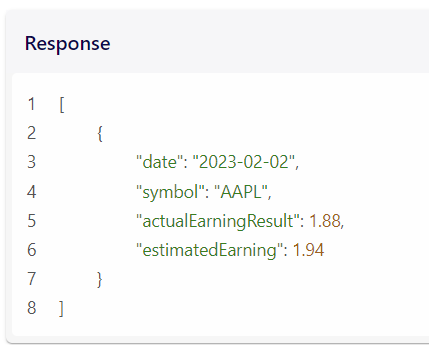
Let’s get the earnings data, parse the JSON and convert it into a DataFrame df_earnings using the code below. We also convert the date column into a Python datetime type and set this as the index so the DataFrame becomes a time series, this is for easier data manipulation later. From the actual earnings and estimated earnings results we will later be able to calculate how much of an earnings surprise there is.

url = f"{base_url}earnings-surprises/{ticker}?apikey={apiKey}"
df_earnings = pd.DataFrame(get_jsonparsed_data(url))
df_earnings['date'] = pd.to_datetime(df_earnings['date']) # changing column to the datetime type
df_earnings = df_earnings.set_index('date') # turn it into time series
df_earnings.head()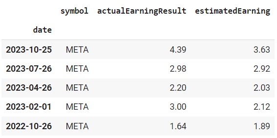

5. Get Stock Prices

This FMP API endpoint https://financialmodelingprep.com/api/v3/historical-price-full/{ticker}?from={earliest_date_string}&apikey={apikey} allows you to get all the stock prices from the earliest date that you want, for any ticker.

A screenshot of the API response from the FMP documentation is shown below.

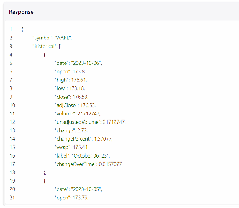
We do not need to get all historical stock prices, but only the one from the earliest earnings date, to eventually perform our correlation later. Hence we get the earliest date of earnings (which is the index of the last row of the df_earnings DataFrame), this is the earliest date from which we will scrape the stock prices. We also need to convert this date into a string to pass to the FMP API url endpoint later.

earliest_date = df_earnings.index[-1] # index of last row is the earliest earnings date in the data
earliest_date_string = earliest_date.strftime('%Y-%m-%d') # convert date to string

Similar to how we obtain the earnings data, we get the prices data, parse the JSON, convert it into a DataFrame df_prices and set the date column as the index.

url = f"{base_url}historical-price-full/{ticker}?from={earliest_date_string}&apikey={apiKey}" # url to scrape prices for ticker, from earliest_date_string
df_prices = pd.DataFrame(get_jsonparsed_data(url)['historical']) # the 'historical' key allows us to get historical prices, see the screenshot of the JSON that the API returns above
df_prices['date'] = pd.to_datetime(df_prices['date'])  # changing column to the datetime type
df_prices = df_prices.set_index('date') # turn it into time series
df_prices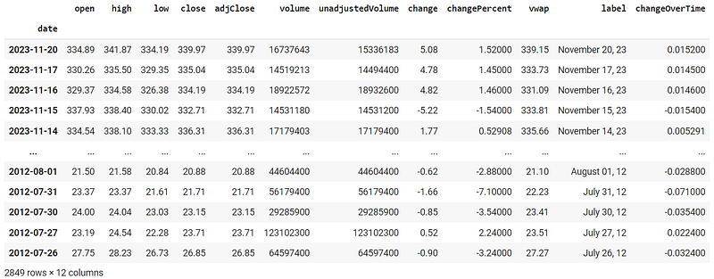

6. Shift the Prices to Correspond to Future Prices

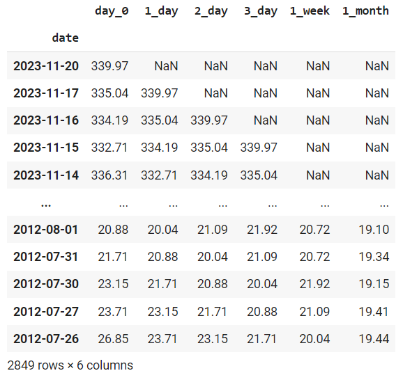
With our stock prices DataFrame, we eventually want to see how the prices change 1 day to 1 month after earnings release. Hence we want to create columns for future prices of the stock. Fortunately, with a time series DataFrame, this process is easy, all we need to do is to use the .shift() method as shown in the code below to shift the prices forward by the number of days we want. Here I shift the time series DataFrame to look at the 1 day, 2 day, 3 day, 1 week and 1 month future prices, feel free to change it to any day you want.

Remember that the days shifted correspond to working days where there is trading (for example, there are about 20 working days in a month, 5 working days in a week, as reflected in the code below. Note that we are using the adjusted close price (adjClose column) for each day to be the stock price. This is the closing price adjusted for things like stock splits etc. throughout history.

df_prices['day_0'] = df_prices['adjClose']
df_prices['1_day'] = df_prices.shift(1)['adjClose']
df_prices['2_day'] = df_prices.shift(2)['adjClose']
df_prices['3_day'] = df_prices.shift(3)['adjClose']
df_prices['1_week'] = df_prices.shift(5)['adjClose'] # 1 week is 5 working days
df_prices['1_month'] = df_prices.shift(20)['adjClose'] # 1 month ~ 20 working days
df_prices[['day_0', '1_day', '2_day', '3_day', '1_week', '1_month']]

In the resulting DataFrame, notice that there are missing rows at the top of each column. For example, the 3_day column of future prices column has 3 missing rows. This is normal because we do not know what the prices are 3 days later, in each of the most recent 3 days as this refers to days in the future (I hope this makes sense!). This means that we may not have enough pricing data to see how the price is affected by the latest earnings results if the releases are too recent. That is fine because our correlation score will be averaged over all historical earnings releases over the whole time period and the missing data will be ignored.

7. Merge the Earnings and Prices Data from the Above Together

Now that we have the both the earnings and pricing data, we can join them together into a DataFrame df by matching them on the index (dates) columns on both DataFrames.

df = df_earnings.merge(df_prices[['day_0', '1_day', '2_day', '3_day', '1_week', '1_month']],
                       left_index = True, right_index = True, how = 'left')

df.head()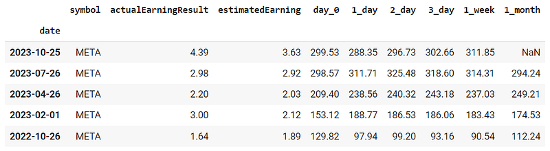

8. Calculate % Difference in Actual Earnings from Estimated Earnings, and % Difference in Future Prices from Current Prices

Having the earnings results and stock prices themselves are not enough, we still need to do a bit of processing as we want to see the correlation between earnings surprises and change in prices.

Here we calculate the % difference in actual earnings vs estimated earnings, and also the % difference in future prices from current prices 1 day, 2 day, 3 day, 1 week and 1 month later using the corresponding future prices columns.

df['earnings_diff'] = (df['actualEarningResult'] - df['estimatedEarning'])/df['estimatedEarning']
df['1_day_diff'] = (df['1_day'] - df['day_0'])/df['day_0']
df['2_day_diff'] = (df['2_day'] - df['day_0'])/df['day_0']
df['3_day_diff'] = (df['3_day'] - df['day_0'])/df['day_0']
df['1_week_diff'] = (df['1_week'] - df['day_0'])/df['day_0']
df['1_month_diff'] = (df['1_month'] - df['day_0'])/df['day_0']

df[['earnings_diff', '1_day_diff', '2_day_diff', '3_day_diff', '1_week_diff', '1_month_diff']].head()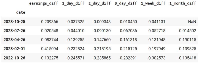

9. Plot % Diff in Future Prices vs % Diff in Expected/Actual Earnings in a Scatterplot

We finally ready to see if there is any correlation between the earnings surprises (% diff in expected/actual earnings) and the price movement (% diff in future/current prices after earnings). Let’s plot these on a scatter for the price difference for each of the different time periods, and fit a regression line to it as well to see if there is any pattern.

plt.rcParams["figure.figsize"] = (10,15)

plt.subplot(3, 2, 1)
sns.regplot(data=df, x="earnings_diff", y="1_day_diff")

plt.subplot(3, 2, 2)
sns.regplot(data=df, x="earnings_diff", y="2_day_diff")

plt.subplot(3, 2, 3)
sns.regplot(data=df, x="earnings_diff", y="3_day_diff")

plt.subplot(3, 2, 4)
sns.regplot(data=df, x="earnings_diff", y="1_week_diff")

plt.subplot(3, 2, 5)
sns.regplot(data=df, x="earnings_diff", y="1_month_diff")

plt.show()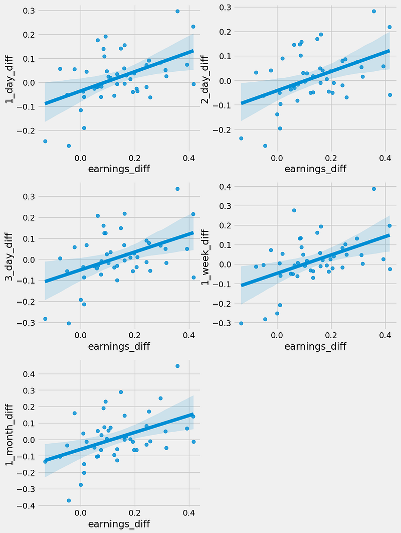

From these plots, it seems like there is indeed some positive correlation between the earnings difference and change in prices after earnings over all the time periods we are interested in (i.e. positive earnings surprises result in positive price changes). At least this is the case for META stock.

10. Calculate Correlation Between the DataFrame Columns, and Plot Out On a Heatmap

Let’s now calculate the correlation between the earnings_diff column and all the price difference columns. We can do this using the .corr() method for the DataFrame as shown below, which returns the correlation score between every pair of columns in the DataFrame in a matrix shown below.

# define color palette, here we define red for negative, green for positive and white for 0
# don't worry too much about this part of the code
rdgn = sns.diverging_palette(h_neg=10, h_pos=130, s=99, l=55, sep=3, as_cmap=True)
divnorm = TwoSlopeNorm(vmin=-1, vcenter=0, vmax=1)

df_corr = df[['earnings_diff', '1_day_diff', '2_day_diff', '3_day_diff', '1_week_diff', '1_month_diff']].corr()
sns.heatmap(df_corr, annot=True, norm=divnorm, cmap=rdgn)

We also plot out the correlation matrix on a heatmap and defined a color palette to use red for negative, green for positive, and white for 0 correlation values. In our case, we only want the first row (or column) (boxed up below) of the matrix as we are not interested in the correlation between the price difference columns themselves.

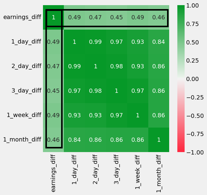
The boxed up values above are all rather positive (all between +0.4 to +0.5), which cannot be ignored. This means there is definitely a rather significant positive correlation, though not a very strong one. This corresponds to what we see on the scatterplots earlier. In the plots, there is a best fit positive sloping line but the points are scattered quite far apart. So there is quite a significant positive correlation in the case for META stock. Is this the same for other stocks as well?

11. Repeat All Steps Above and Put the Code Together for Different Tickers

The following code loops through multiple tickers of interest (feel free to change the list of tickers to your favorite ones), repeats all the above steps and extracts the first row of the correlation matrix. Then it combines all these rows together into a final DataFrame df_all of correlation scores between earnings surprises and price movement for each time period, for each ticker.

tickers = ['GOOG', 'META', 'AAPL', 'MSFT', 'NVDA', 'NFLX', 'V', 'MA', 'AMZN',
 'TSLA', 'JPM', 'BAC', 'C', 'BA', 'MMM', 'HON', 'CRM', 'PLTR', 'VEEV', 'JNJ', 'HCA', 'UNH', 'BABA']

df_all = pd.DataFrame() # to store results for all tickers

for ticker in tickers:
    print("Scraping Earnings Surprises and Stock Prices for", ticker)

    # scrape earnings surprises from FMP API
    url = f"{base_url}earnings-surprises/{ticker}?apikey={apiKey}"
    df_earnings = pd.DataFrame(get_jsonparsed_data(url))
    df_earnings['date'] = pd.to_datetime(df_earnings['date'])
    df_earnings = df_earnings.set_index('date')

    # scrape stock prices from FMP API
    earliest_date = df_earnings.index[-1]
    earliest_date_string = earliest_date.strftime('%Y-%m-%d')
    url = f"{base_url}historical-price-full/{ticker}?from={earliest_date_string}&apikey={apiKey}"
    df_prices = pd.DataFrame(get_jsonparsed_data(url)['historical'])
    df_prices['date'] = pd.to_datetime(df_prices['date'])
    df_prices = df_prices.set_index('date')
    df_prices['day_0'] = df_prices['adjClose']
    df_prices['1_day'] = df_prices.shift(1)['adjClose']
    df_prices['2_day'] = df_prices.shift(2)['adjClose']
    df_prices['3_day'] = df_prices.shift(3)['adjClose']
    df_prices['1_week'] = df_prices.shift(5)['adjClose']
    df_prices['1_month'] = df_prices.shift(20)['adjClose']

    # merge the data
    df = df_earnings.merge(df_prices[['day_0', '1_day', '2_day', '3_day', '1_week', '1_month']],
                           left_index = True, right_index = True, how = 'left')
    df['earnings_diff'] = (df['actualEarningResult'] - df['estimatedEarning'])/df['estimatedEarning']
    df['1_day_diff'] = (df['1_day'] - df['day_0'])/df['day_0']
    df['2_day_diff'] = (df['2_day'] - df['day_0'])/df['day_0']
    df['3_day_diff'] = (df['3_day'] - df['day_0'])/df['day_0']
    df['1_week_diff'] = (df['1_week'] - df['day_0'])/df['day_0']
    df['1_month_diff'] = (df['1_month'] - df['day_0'])/df['day_0']

    # calculate correlation
    df_all[f'{ticker}'] = df[['earnings_diff', '1_day_diff', '2_day_diff', '3_day_diff',
                                            '1_week_diff', '1_month_diff']].corr()[['earnings_diff']]

df_all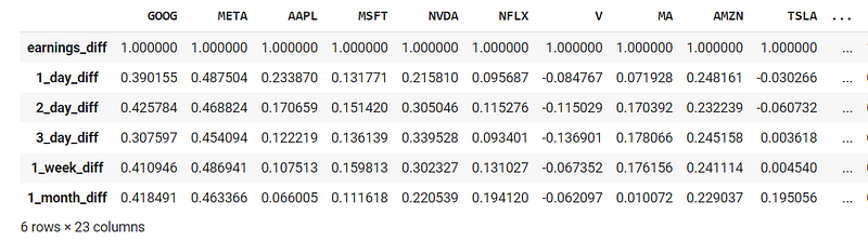

We then sort the order of the summary DataFrame of correlation scores by the 1_day_diff correlation with the earnings surprises, starting from highest to lowest. We also calculate the average correlation scores for each ticker in the final row and rename the DataFrame df_summary.

df_summary = df_all.T
df_summary = df_summary.iloc[:, 1:]
df_summary = df_summary.sort_values('1_day_diff', ascending = False)
df_summary.loc['Average'] = df_summary.mean()
df_summary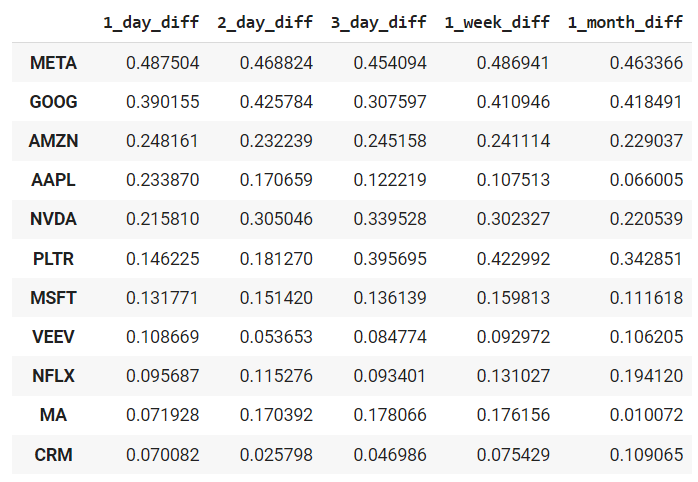

12. Heatmap Plot of Correlation Between Earnings Surprises and Stock Price Movements

Next, we plot the above summary DataFrame into a heatmap, using the same color scheme as defined earlier (red for negative, green for positive, and white for 0 correlation values).

rdgn = sns.diverging_palette(h_neg=10, h_pos=130, s=99, l=55, sep=3, as_cmap=True)
divnorm = TwoSlopeNorm(vmin=-0.5, vcenter=0, vmax=0.5)

plt.rcParams["figure.figsize"] = (16,8)
plt.title('Heatmap Plot of Correlation Between Earnings Surprises and Stock Price Movements')
sns.heatmap(df_summary, annot=True, norm=divnorm, cmap=rdgn)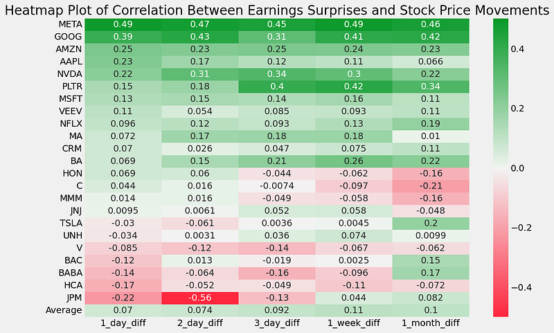

Here we can see that the magnificent 7 stocks (e.g. META, GOOG, AMZN, AAPL, NVDA, MSFT, except for TSLA) are among the top few positive ones in terms of correlation between earnings surprises and stock price movements. This is not surprising as I assume that there will be many news articles written on these companies whenever they release earnings. There may be many people trading these companies as well. These people may be eager about their results and respond accordingly to buy/sell the stocks whenever they have positive/negative earning surprises.

The healthcare and defensive stocks (e.g. HON, MMM, JNJ, UNH) are in the middle rows, meaning they have very small correlation values (neither positive nor negative). This is also expected as prices of defensive stocks tend to be more stable and perhaps more people invest in the stocks long term to hold through both good and tough times rather than trade them. Their earnings may tend to be more predictable and stable, hence the reaction to the earnings may not be as strong.

Interestingly the bank stocks (e.g. BAC, JPM) have negative correlation scores. Perhaps people always expect even more earnings even if they beat the expected earnings, resulting in a sell down anyway? I am not sure!

But I’m sure some of you would have observed these days that China stocks like BABA seem to have good fundamentals and produce positive earnings beat, yet sadly continue to have their stock prices beaten up. This is reflected in our heatmap above in that BABA is indeed in one of the last few rows with a negative correlation between earnings surprises and price movements!

Conclusion

Hopefully, this article has allowed you to more quantitatively determine if earnings surprises correlate to stock price movements, and for which stocks are there stronger/weaker or even negative correlations. Feel free to try the code out and edit it to run on your favorite stocks instead. These correlation scores may also be useful input features if you are trying out any model to predict stock prices after earnings. Have fun!

The actual and estimated earnings data as well as the stock prices from the above are scraped from the Financial Modeling Prep API, which is an accurate financial data (i.e. stocks, earnings, historical data, market sentiment, financial statements etc.) API. Once again, you can sign up for it at a discounted rate here, there is a free version too.

If you enjoyed this article, feel free to check out my other articles below and feel free to follow me. :)

Linkedin: https://www.linkedin.com/in/damian-boh/

Visit us at DataDrivenInvestor.com

Subscribe to DDIntel here.

Have a unique story to share? Submit to DDIntel here.

Join our creator ecosystem here.

DDIntel captures the more notable pieces from our main site and our popular DDI Medium publication. Check us out for more insightful work from our community.

DDI Official Telegram Channel: https://t.me/+tafUp6ecEys4YjQ1

Follow us on LinkedIn, Twitter, YouTube, and Facebook.