Is the Trend Your Friend? A Survey of the Persistence of Returns, by Year

The Autocorrelation of NASDAQ–100 Member Returns

In a prior article here on Medium, I showed how to compute a benchmark reference table for scoring the performance of machine learning algorithms that purport to predict the performance of NASDAQ–100 stocks. That was done by demonstrating how much of the variance of their prices is explained by simply the prior day’s price.

Results for Predicting the Prices of NASDAQ–100 using Just the Prior Day’s Price

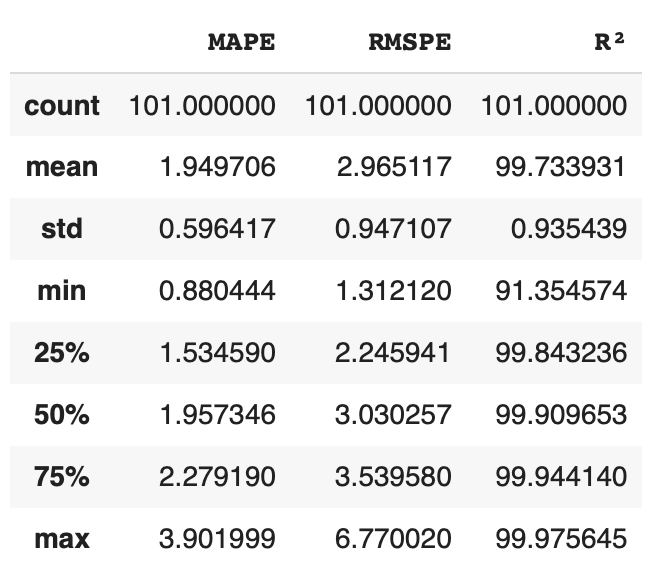
It’s important to note that the purpose of that investigation was not to assert that you should trade on the idea that yesterday’s price provides a useful forecast of today’s price. It is a fairly accurate forecast, but it is not a useful one. That is because you cannot make money from it: it tells you that your expected return is zero. Even if we believe in completely efficient markets, we know your expected return is not zero — it is positive and proportional at some level to the amount of systematic risk you take on as a trader.

I do, however, like the idea of systematically surveying some asserted property of markets and comparing the results year-on-year. This is aligned with several things I think are true:

1. real alphas do exists;
2. parameterizations are not stationary.

Momentum and Correlation

“The trend is your friend” is a saying thrown around on trading desks. It says that “momentum” exists in the markets, and that you should embrace it rather than fight it if you want to make money. As a quant, though, what does “momentum” actually mean?

In classical physics, momentum is a quantification of the property that a mass in motion tends to stay in motion unless it is acted upon by an external force. What in econometrics would be described as an exogenous factor. Parsing that into the time-series properties of the prices of securities, we tend to say that tomorrow’s returns will be aligned with today’s returns. That is there is an autoregression for returns, which is written as

This equation means that the expected value of tomorrow’s return of stock i,when conditioned on information available today, is proportional to today’s observed return of the stock. If Apple went up today it is more likely to go up tomorrow than go down, and if Tesla went down today it is more likely to continue to go down tomorrow than to go up.

To model stocks we need to take account of other factors, such as the general upwards drift of stocks and other systematic risk factors that are viewed as generally unpredictable in magnitude but that influence the cross-sectional covariance of returns, which is the fact that Apple and Amazon tend to go up and down on the same day. The simplest way to do that is the linear additive noise model, which asserts that the prior relationship can be encoded as something like

This expression makes the same statement, that tomorrow’s returns of stock i will be found to be proportional to today’s returns. In the model μ represents a general bias in returns (found to be positive over the long run) and ε is encapsulating everything that is unpredictable. What is left is the term directly proportional to today’s return.

If the coefficient, φ, is positive this represents momentum, or trending, as it says the positive returns are more likely to deliver subsequent returns of the same sign, and if it is negative it represents mean reversion, as it indicates that an outsized positive return is more likely to be followed by a negative return for the same stock — that big moves upwards are subsequently reversed and that the same applies to big moves downwards.

Autoregression is Autocorrelation

The prior expression is called an “auto-regression” because it is a linear regression equation in which the dependent variable and the independent variable are the same thing, apart from the time lag between them. It is regressed onto itself. However, there is another feature of that expression which is that it entirely determines what the correlation coefficient between today’s return and tomorrow’s return should be. It is simple to show that

thus, if the linear additive noise model is true, the regression coefficient of sequential returns must lie somewhere between –1 and +1. It is their correlation.

Pearson’s r and Other Measures of Association

The “correlation” referred to above is more formally known as Pearson’s r or the product moment coefficient. It is the measure computed as

when x and y have a joint probability density f(x,y). For many it is the first non-trivial “statistic” that they learn about in high-school math.

Ordinal Correlation Measures

Pearson’s r, when first introduced in the 1880’s based on the work done by Sir Francis Galton on heredity and the concept of “regression to the mean,” was groundbreaking and Pearson had a substantial influence on the foundations of Statistics from his position at University College, London.

Like many of that era, he was applying the newly created statistical science to matters of human development, which we must not forget included the study of eugenics.

It was known from at least the work of Charles Spearman, that Pearson’s r was problematic when applied to data that could be ranked but for which the magnitude of the measure was not important. Spearman introduced a “rank correlation,” which is often suitable for use when what’s important is the total ordering of compared measures, and many will have heard of this — although it is seldom used in data science.

Later on, Sir Maurice Kendall introduced the concept of the concordance and discordance of relative rankings of data. He was working in the field of social science where measures of a population were often graded on a simple scale of 1 to 5 and he wanted to assess the manner in which two measures tended to agree or disagree. He introduced a measure, now called Kendall’s τ, which for two sets of data is computed as the number of pairs (x,y) where the ordering of pairs of values of x and y agree minus the number of pairs where those orderings of pairs of values disagree all divided by the total number of possible pairs. This sounds complicated, but it’s actually quite simple. It’s a statement about the agreement of the sorting orders of the two data-sets.

This says nothing about the relative magnitudes of the data, which dominates the computation of Pearson’s r, and is entirely focussed on their tendency to have similar sorting orders. As such it is a measure which, despite being introduced in the 1930’s, is eminently suitable for use in 21st. century data science as it is a robust measure of association that doesn’t require the introduction of a linear model or the Normal distribution to understand its properties.

Surveying Kendall’s Rank Correlation for the Returns of NASDAQ–100 Stocks

As I stated in the beginning of this article, I am very interested in the global properties of the returns of stocks. Let’s take a look at whether there’s an ordinal relationship between yesterday’s return and todays return of the members of the NASDAQ–100 Index.

As before, let’s start with a Colab project to download the members of the index.

print("Installing yfinance and getting data...")
!pip install yfinance 1>/dev/null
import pandas as pd
import numpy as np
from yfinance import download
from datetime import datetime

# set time frame of analysis
today=datetime.now()
last_year=today.year-1
prior_year=today.year-2

# this list as of 2020-12-21
# you must use Adjusted Close to account for distributions such as
# dividends and splits, not simple Close
prices=download(['AAPL','ADBE','ADI','ADP','ADSK','AEP','ALGN','AMAT','AMD','AMGN','AMZN','ANSS','ASML','ATVI','AVGO','BIDU','BIIB','BKNG','CDNS','CDW','CERN','CHKP','CHTR','CMCSA','COST','CPRT','CRWD','CSCO','CSX','CTAS','CTSH','DLTR','DOCU','DXCM','EA','EBAY','EXC','FAST','FB','FISV','FOXA','GILD','GOOG','GOOGL','HON','IDXX','ILMN','INCY','INTC','INTU','ISRG','JD','KDP','KHC','KLAC','LRCX','LULU','MAR','MCHP','MDLZ','MELI','MNST','MRNA','MRVL','MSFT','MTCH','MU','NFLX','NTES','NVDA','NXPI','OKTA','ORLY','PAYX','PCAR','PDD','PEP','PTON','PYPL','QCOM','REGN','ROST','SBUX','SGEN','SIRI','SNPS','SPLK','SWKS','TCOM','TEAM','TMUS','TSLA','TXN','VRSK','VRSN','VRTX','WBA','WDAY','XEL','XLNX','ZM'],"%d-01-01" % prior_year,"%d-12-31" % last_year)["Adj Close"]

# this is to make sure the index is properly time aware
prices.index=pd.DatetimeIndex(prices.index).to_period('D') 
prices

This gets the daily adjusted closing prices for the members of the index as of the end of 2020, and it gets them for data from the start of 2020 to the end of 2021. This is so that we can conduct an experiment as follows:

1. get the index members as of year end
2. compute the autocorrelation of their returns for the prior year
3. compare these values to the the returns of the same stocks for the next year.

Doing it this way, we are survivorship bias free and this replicates actual behaviour that a trader could engage in, it just shows us the results “as if” we’d done this analysis a year ago.

The next thing to do is to compute returns:

# make returns
returns=pd.DataFrame({
    ticker:prices[ticker]/prices[ticker].shift()*1e2-1e2 \
         for ticker in list(prices)
})
returns["Year"]=list(map(lambda x:x.year,list(returns.index)))
returns

This uses a dictionary comprehension to construct a new data-frame from the downloaded prices, and adds an indicator variable for the year of the data.

Finally, we compute Kendall’s τ ticker-by-ticker for daily returns and the prior day’s returns, for each year of data collected.

# compute Kendall's Tau for concordance of daily returns by ticker
kendall=pd.DataFrame({year:[np.nan]*prices.shape[1] \
    for year in [prior_year,last_year]})
kendall["Ticker"]=list(prices)
kendall.set_index("Ticker",inplace=True)

for ticker in prices:
    for year in kendall:
        selection=returns["Year"]==year
        correlation=pd.DataFrame({
            "return":returns.loc[selection,ticker],
            "prior_return":returns.loc[selection,ticker].shift()
        }).dropna().corr(method='kendall')
        kendall.loc[ticker,year]=\
              correlation.loc["return","prior_return"]

kendall

Do Returns show Momentum in 2020?

Hypothesizing that we were back at the end of 2020, trying to see if we should be a momentum or reversion trader in 2021, we want to measure the rank correlations, or concordance, of the stocks in the index ticker-by-ticker. That is the data Kendall[2020] in the data-frame constructed. A simple histogram is worth looking at:

Kendall[2020].hist(bins=np.linspace(-0.2,0.1,25));

The notebook linked to makes a slightly more complex plot, which looks like this:

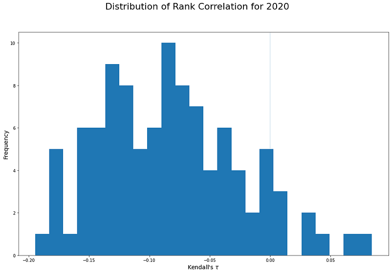
This shows that, stock-by-stock, for 2020 in a Universe chosen at the end of 2020, returns tend to be discordant with the prior day’s returns. The distribution is right skewed with a mean of –8%, and this is quite a significant result (p value for a mean of zero is vanishingly small).

Looking back at 2020 from the end of the year, if you had picked a stock at random it probably would not have exhibited momentum during that year. Note that, in interpreting the data this way, we have removed the effect of the drift of stocks during the analysis period. Many stocks did, in fact, show strong upward movement through 2020 as a whole, but this analysis is about looking at each day’s return and using it as a trading signal for the day that follows. On that basis, you should have faded the trend, not followed it.

Is the Distribution of Correlations Stable?

Projecting ourselves back to the beginning of 2021, and armed with the information that daily returns were discordant for most stocks in the NASDAQ–100, what can we do with that information? A necessary condition for such information to be an input to a profitable trading system would be that the returns would have a similar property in the following year.

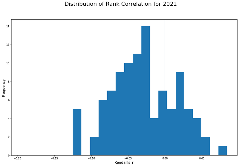
Now things become interesting. As a whole the statement is the same: stock-by-stock returns were discordant during 2021, this time the distribution has a mean of –3%, and more stocks exhibit momentum than for the prior year. Specifically, though, there are plenty of stocks where reversion trading based on the correlations of daily returns would have led to losses in the following year.

Do 2020’s Correlations Predict those for 2021?

What’s really interesting, then, is to look at whether the correlations as measured at the end of 2020 were useful indicators of correlations for the same stock for the following year. That is, if we had filtered this list by the stocks with the strongest correlations for each year would each year’s list contain the same stocks?

Again this can be done very straightforwardly:

kendall.plot.scatter(prior_year,last_year)

Again, the notebook makes a more detailed plot.

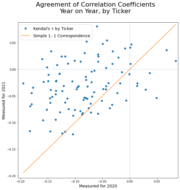
This is very interesting as it shows that most of the NASDAQ–100 stocks had similar correlations of returns for both 2020 and 2021. So a trader who had used 2020’s data to build strategies for trading in 2021 would have probably prospered in that year despite the fact that the specific values of the correlations changed and that, for 27% of the index, the sign itself was different.

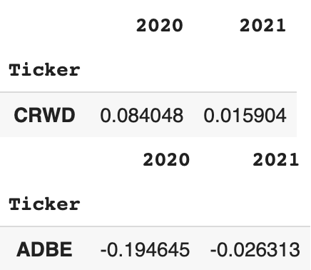
Furthermore both the stock with the most positive correlation, $CRWD, and that with the most negative correlation, $ADBE, both had the same signed correlation in the following year — although the magnitudes were much lower.

If you like this article and would like to read more of my work, consider my book Adventures in Financial Data Science which is available as an eBook for Kindle, and also from Apple Books and Google Books. A revised second edition will be published by World Scientific.

Alternatively, you can order the paperback directly from me via our website.

You can directly support my writing on Medium by subscribing through this affiliate link.

And if you want to chat with me about my work, consider joining our slack channel.