Price Optimization: Is the Price Right? using Machine Learning Approach

In the dynamic world of business, setting the right price for products and services is more than just a matter of guesswork or following the industry norm. Price Optimization stands at the forefront of a company’s strategy, serving as a crucial lever to enhance profitability, competitiveness, and customer satisfaction. This delicate balancing act involves determining the optimal price point that maximizes business objectives, be it revenue, market share, or profit margins.

In traditional settings, pricing strategies were often guided by a combination of historical data, competitor pricing, and gut feeling. However, in today’s data-driven era, Machine Learning (ML) has revolutionized this approach. By harnessing the power of ML, businesses can analyze vast amounts of data — encompassing past sales figures, customer behavior patterns, market trends, and even competitor activities — to make informed, strategic pricing decisions.

The Transformative Role of Machine Learning in Price Optimization

Machine Learning (ML) has revolutionized price optimization, shifting it from intuition-based to data-driven decision-making. By analyzing vast datasets, ML uncovers intricate patterns in consumer behavior, market trends, and competitive dynamics. This deep insight allows businesses to predict how different pricing strategies might play out, enabling them to adjust their pricing models in real time for optimal outcomes. From automating routine pricing decisions to offering personalized pricing strategies, ML empowers businesses to not only respond swiftly to market changes but also to proactively shape their pricing tactics in line with overarching business goals. The result is a significant enhancement in both competitiveness and profitability, making ML an indispensable tool in modern price optimization strategies.

Understanding the Dataset: Insights from a Cafes Sales

Our analysis revolves around a dataset from a cafe known for its select offerings: Burgers, Coke, Lemonade, and Coffee. This dataset is a window into the café’s sales dynamics, providing valuable insights into customer preferences and the effectiveness of different pricing strategies. Here’s an overview of the key variables that form the core of our analysis:

• Date: This variable marks the date of each transaction, vital for uncovering sales trends, seasonal preferences, and customer visit patterns over time.
• Price: The sale price of each item, pivotal in understanding how pricing adjustments influence sales volumes and overall revenue for the café’s limited but popular menu items.
• Quantity (qty): The number of units sold for each item, a direct indicator of customer demand and the popularity of each menu offering.
• Seller ID (sell_id): A unique identifier for each transaction or sales point, important for tracking sales performance across different counters or service points within the café.
• Seller Category (sell_cat): Classifies the type of sale (e.g., dine-in, take-away, online order), providing insights into the most preferred modes of purchasing by the customers.
• Item: Identifies the product sold (Burger, Coke, Lemonade, Coffee), essential for assessing which items are the bestsellers and understanding the product-specific demand patterns.
• Year: The year of the sale, useful for examining annual trends and changes in customer behavior over time.
• Holiday: Indicates whether a sale was made on a holiday, a factor that can significantly influence café visitation and consumption patterns.
• Is Weekend (is_weekend): A binary indicator denoting whether the transaction was during the weekend, crucial for understanding weekend versus weekday sales trends.
• Is School Break (is_schoolbreak): Reflects whether the sale occurred during a school vacation period, which can affect the café’s footfall and sales, especially if it is located near educational institutions.
• Average Temperature (avg_temperature): Offers context on the weather conditions, which can impact customer preferences, especially for beverages like Coke and Lemonade.
• Is Outdoor (is_outdoor): Shows whether the sale was made in an outdoor setting of the café, relevant for understanding the preference for dining environments among customers.

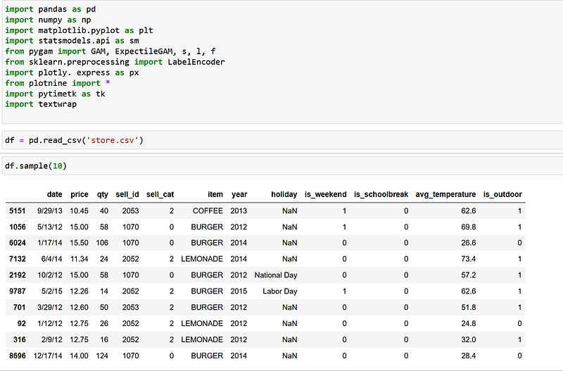
We will start by importing the libraries, loading and analysing few rows from the dataset.

Let’s explore the variety of items included in the dataset to understand the range of products the café offers.

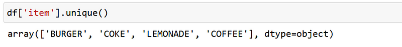
The dataset consist of four distinct items offered by the cafe: Burger, Coke, Lemonade, and Coffee.

Check if dataset has any missing values

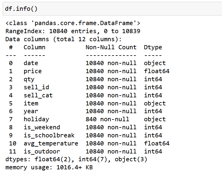
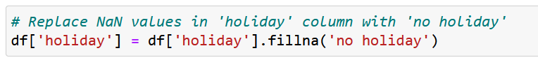
The ‘holiday’ column in the dataset contains 10,000 NAN entries, which essentially represent instances of ‘no-holiday’. Therefore, these missing values will be filled in with the label ‘no_holiday’ for clarity and accuracy in the data.

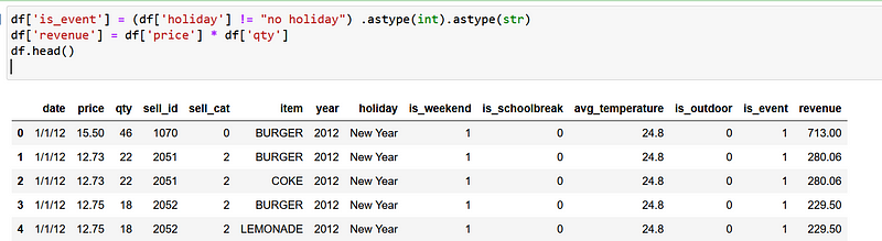
To enhance our analysis, new columns have been added to the dataset. The ‘is_event’ column is created, where a value of ‘1’ indicates days corresponding to holidays, as per the ‘holiday’ column. Additionally, a ‘revenue’ column is introduced, calculated as the product of ‘price’ and ‘qty’, representing the total revenue from each sale. The first few entries of the modified dataset are displayed below to illustrate these changes.

Data Analysis Exploration

Our focus will be on examining how prices and quantities sold are influenced by various features within the dataset.

How does the average price of items vary over the years?

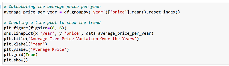
The line plot, which illustrates the variation in average item prices over several years, shows an initial increase in prices from 2012 to 2014, followed by a downward trend in subsequent years.

Is there a notable difference in the quantity sold during holidays compared to non-holidays at different price points?

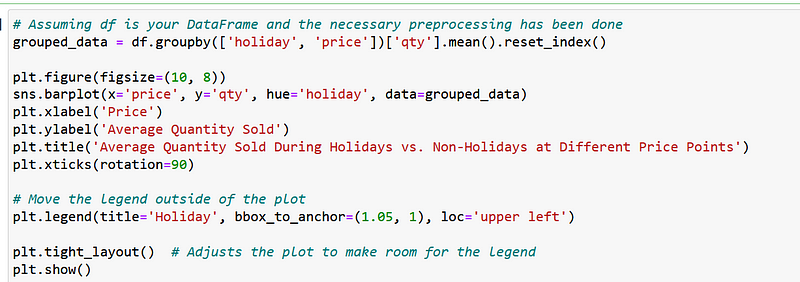
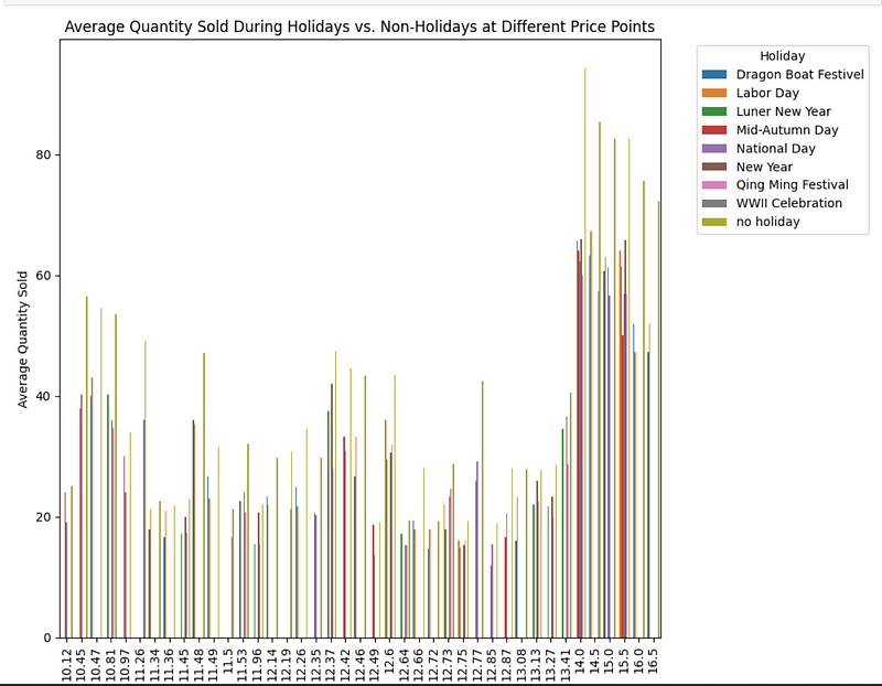
The bar chart effectively demonstrates that, across various price points, the average quantity sold during non-holiday periods surpasses that during holidays.

Does the weekend influence the quantity sold at varying prices?

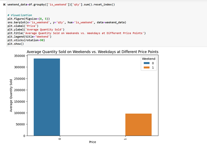
It is clearly visible that the quantity sold on weekdays surpasses that sold on weekends.

Is there a Impact of School breaks on Quantity sold

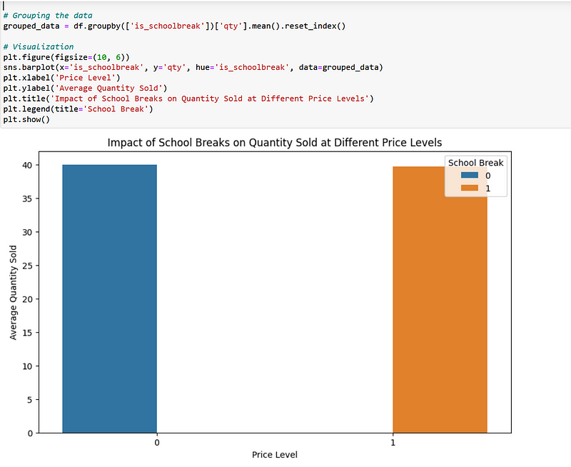
The quantity sold remains unaffected by school breaks, indicating that sales are consistent regardless of whether it is during a school session or a break.

How do sales quantities differ across items?

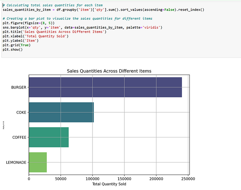
The bar chart reveals that the total quantity of burgers sold is twice that of any other item, with Coke, coffee, and lemonade trailing behind, the latter having the lowest sales quantity.

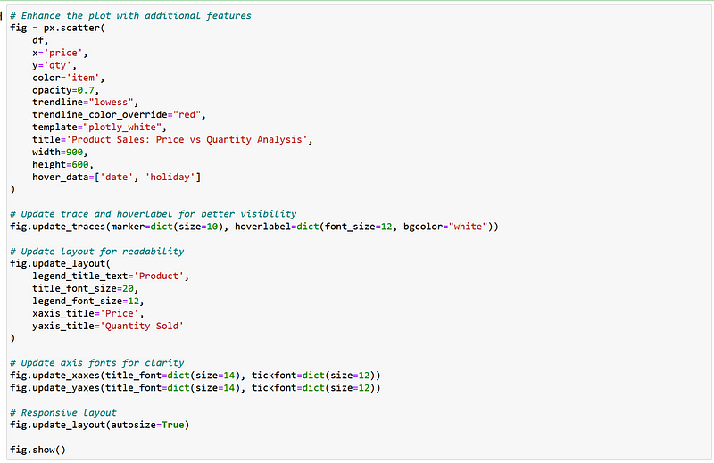
Continuing with our primary focus on price optimization, we’ll examine how both quantity and price fluctuate across various items using the below graph. This analysis will provide insights into the dynamics of pricing and sales volumes for different products.

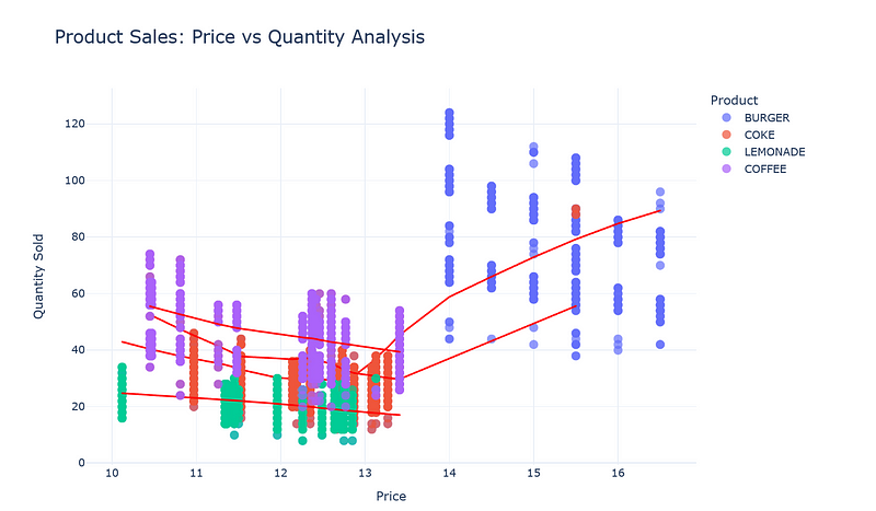
From the above graph its clear the burger prices have range from $10 to $16.5, coke(orange points)ranges from $10 to $15.5, Lemonade(green points) coffee (violet points) ranges from $10 to $13

When the price of burgers rises, there is a noticeable trend of increasing demand, with the price hike having a relatively minor impact. In contrast, for lemonade, coke, and coffee, an increase in price results in a decrease in demand. This observation serves as an initial step in determining the optimal pricing strategy.

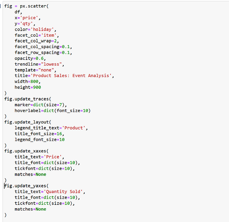
Let’s take a step further and examine how both price and demand fluctuate in response to various types of holidays.

The demand during non-holidays, as indicated by the orange line, is higher when compared to the demand during holidays.

Let’s simplify the visualization by filtering out the data for non-holiday and Labor day.

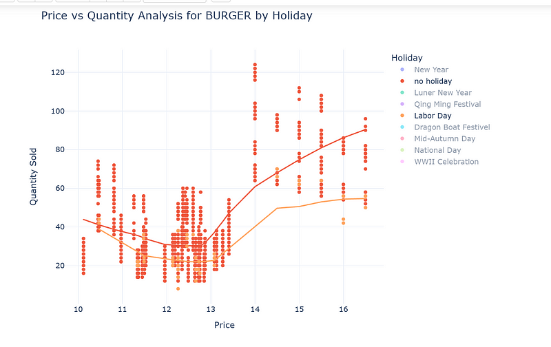
The provided graph illustrates the relationship between the price of burgers and the quantity sold, differentiated by holiday occurrences. The trend line for non-holiday periods shows a gradual downward slope, indicating that as prices increase, the quantity sold tends to decrease, which is a typical demand curve in economics suggesting some degree of price sensitivity. However, the dense clustering of data points around the middle price range could imply a level of price elasticity where sales volume remains relatively stable despite price fluctuations. This area represents an optimal pricing zone where businesses might experiment with price adjustments without significantly impacting sales volume.

In contrast, the trend line for Labor Day, represented in orange, suggests a steeper decline in the quantity sold as prices increase, signifying a higher sensitivity to price changes during this particular holiday. This indicates that consumers might be less willing to purchase burgers at higher prices on Labor Day compared to other days. For effective price optimization, businesses should consider these behavioral changes and potentially adopt a more conservative pricing strategy during holidays to maintain sales volume.

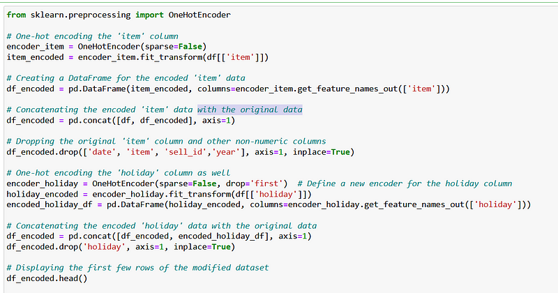
Categorical Encoding

In this section , we apply one-hot encoding to the ‘item’ and ‘holiday’ columns, converting categorical variables into a numerical format without dropping the first category, to fully retain the information for modeling purposes. This encoding expands our dataset with binary columns for each category, enabling it to accommodate machine learning algorithms that require numerical input.

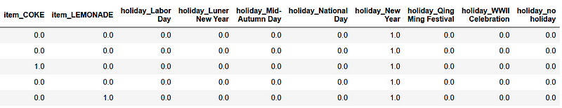
Analyzing the first few rows after encoding:

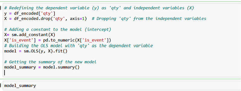
Building a Model Using OLS

We will apply Ordinary Least Squares (OLS) regression model with qty as the dependent variable to understand the influence of each independent variable on the quantity sold. By fitting the model and retrieving the summary, we gain valuable insights into the relationships within our data, which will guide our strategies for price optimization and sales forecasting. This model summary is pivotal in our data analysis journey, as it lays down the statistical foundation for interpreting how various factors affect sales.

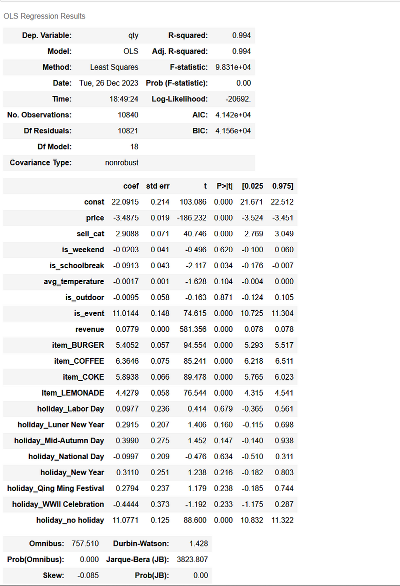
The OLS (Ordinary Least Squares) regression results shown in the image provide a detailed summary of the model that predicts the quantity sold qty based on various features.

• The R-squared value is 0.994, indicating that the model explains 99.4% of the variability in the dependent variable, which is a very high value and suggests a good fit of the model to the data.
• The Adj R-Squared is also 0.994, which adjusts for the number of predictors in the model, indicating a similarly good fit after accounting for the number of variables.
• The coef column shows the estimated value for each coefficient in the regression equation. For example, for each one-unit increase in price, there is an average decrease of 3.4875 units in the quantity sold, holding all other factors constant.

To make it to simple to understand, I will draw comparisons about the sales quantities of burgers and coffee during non-holiday periods versus New Year

For Burgers:

• The coefficient for item_BURGER is significantly positive, indicating that burgers generally contribute positively to sales quantities.
• The holiday_no_holiday coefficient is positive and significant, suggesting higher sales for burgers during non-holiday periods compared to the average holiday.
• There is no specific coefficient for burgers during New Year, but the holiday_New Year coefficient is not significant, implying that the New Year holiday does not have a statistically significant impact on burger sales compared to other holidays.

Price Optimization for Burgers:

• Since burgers sell better during non-holiday periods, a pricing strategy could include maintaining or slightly increasing prices during these times, assuming demand is less sensitive to price changes.
• During New Year, when the data does not indicate a significant increase or decrease in sales, maintaining the price or using promotional deals could be beneficial to attract customers who are celebrating the holiday.

For Coffee:

• Similar to burgers, item_COFFEE has a positive coefficient, showing that coffee is also a strong seller.
• Again, holiday_no_holiday being positive indicates that coffee, too, enjoys higher sales during non-holiday times.
• As with burgers, there is no specific coefficient for coffee during New Year, and the holiday_New Year coefficient is not significant, suggesting no significant difference in coffee sales during New Year compared to other holidays.

Price Optimization for Coffee:

• Since coffee also tends to sell more during non-holiday periods, the pricing strategy for coffee could parallel that of burgers — keeping prices steady or slightly higher when demand is consistent.
• For the New Year, without evidence of a sales increase or decrease, coffee prices might be kept stable to maintain sales, or special New Year promotions could be considered to capture the festive market.

Conducting the Analysis

In this section, we delve into the process of applying Expectile Generalized Additive Models (GAM) to our sales data, focusing on how different pricing strategies might influence quantities sold and, consequently, revenue generation.

Expectile Generalized Additive Models (GAMs) offer a sophisticated approach to understanding data, particularly effective in pricing analysis. Unlike conventional models that focus on average outcomes, Expectile GAMs can predict outcomes at specific quantiles, such as the 2.5th, 50th, and 97.5th percentiles. This feature is particularly useful in pricing analysis, as it allows us to explore not just the most common outcomes but also the variations and extremes, providing a comprehensive understanding of how different pricing strategies might perform under varying market conditions.

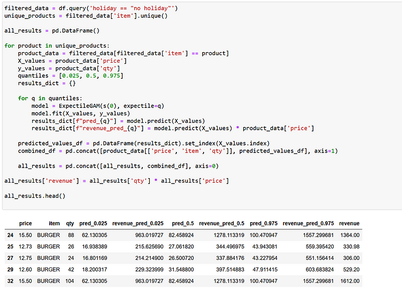
Our analysis begins by filtering the dataset to focus on non-holiday sales periods, as indicated by the ‘holiday’ column. This step is crucial to isolate regular sales patterns, unaffected by the seasonal spikes often associated with holidays.

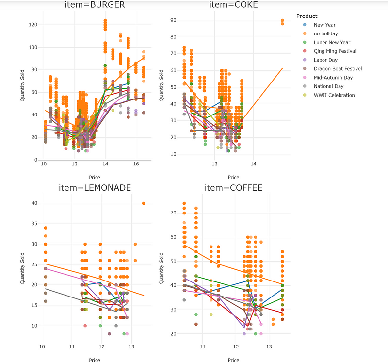
Let’s visualize the relationship between price and quantity sold for different items, including predictive lines and percentiles, while also comparing different items in separate facets.

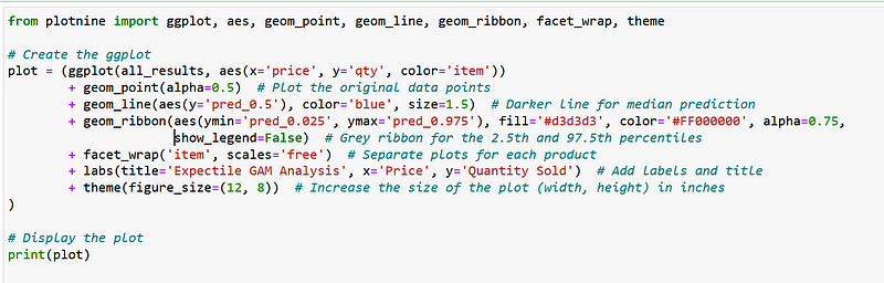
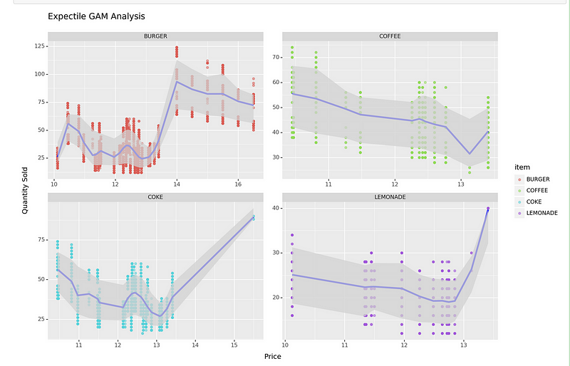
From above visualization we can infer that the relationship between price and quantity sold varies by item.

• Burgers: There is a non-linear relationship with a somewhat volatile quantity sold at different prices, showing peaks and troughs. The quantity sold seems to peak at mid-range prices before declining as prices increase further.
• Coffee: There is a general downward trend in the quantity sold as the price increases, with a slight increase at the higher end of the price range, suggesting a premium pricing effect.
• Coke: The quantity sold appears to increase with the price after a certain threshold, suggesting that higher prices may convey a sense of higher quality or value.
• Lemonade: There is a downward trend in the quantity sold as the price increases, suggesting price sensitivity for this item.

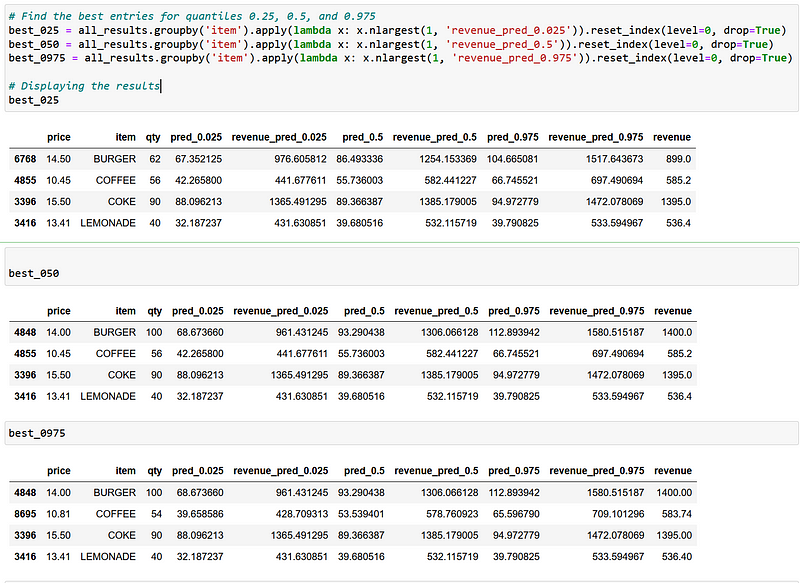
Identifying Optimal Entries for Different Quantiles

In this section, we are interested in finding the best entries for specific quantiles: 0.025, 0.5, and 0.975. These quantiles represent different levels of expectations or predictions.

Quantile 0.025 (2.5th Percentile): This quantile corresponds to a lower expectation, and we want to find the entry or product that generates the highest revenue prediction at this level.

Quantile 0.5 (50th Percentile): This quantile represents the median or middle expectation. We aim to identify the entry or product that performs best in terms of revenue prediction at this level.

Quantile 0.975 (97.5th Percentile): This quantile corresponds to a higher expectation, and we are looking for the entry or product with the highest revenue prediction at this level.

Next, we will create scatter plots with predictive modeling for price optimization of various items burgers, coffee, coke, and lemonade. Each plot corresponds to one item and shows the relationship between price and revenue. The data points represent observed or simulated revenue values at different prices.

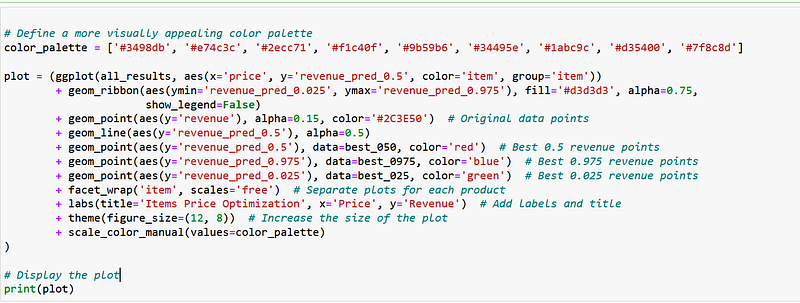
The plots also show predictive confidence intervals (the shaded areas), which give an idea of the range within which the true revenue values are expected to fall with a certain level of confidence.

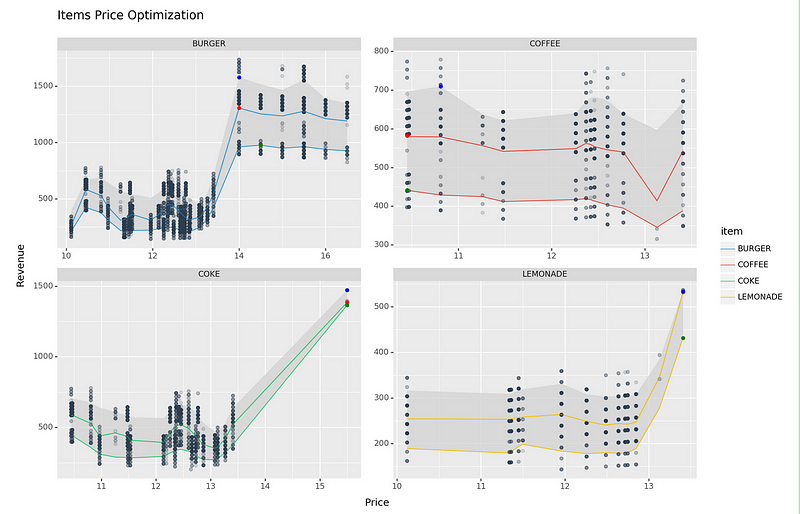
Interpretation for each item:

1. Burger: The red dot, which indicates the optimal price point with the highest median predicted revenue, is placed at around a price point of 14 which will be the best price and will yield maximum revenues.
2. Coffee: The optimal price point for coffee is around a price point of $10
3. Coke: The optimal price for coke is over $15
4. Lemonade: For lemonade, the red dot is situated at a price point of over $13.

These observations suggest that, within the price range analyzed, both Coke and Lemonade could potentially see increased revenue if their prices are raised.

We will further analyse the best price for different holidays.

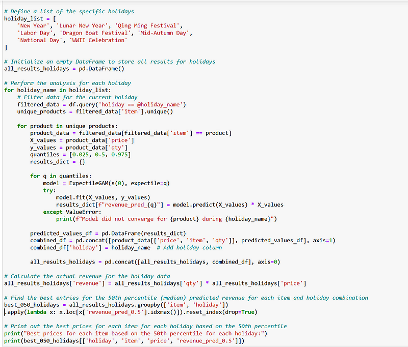
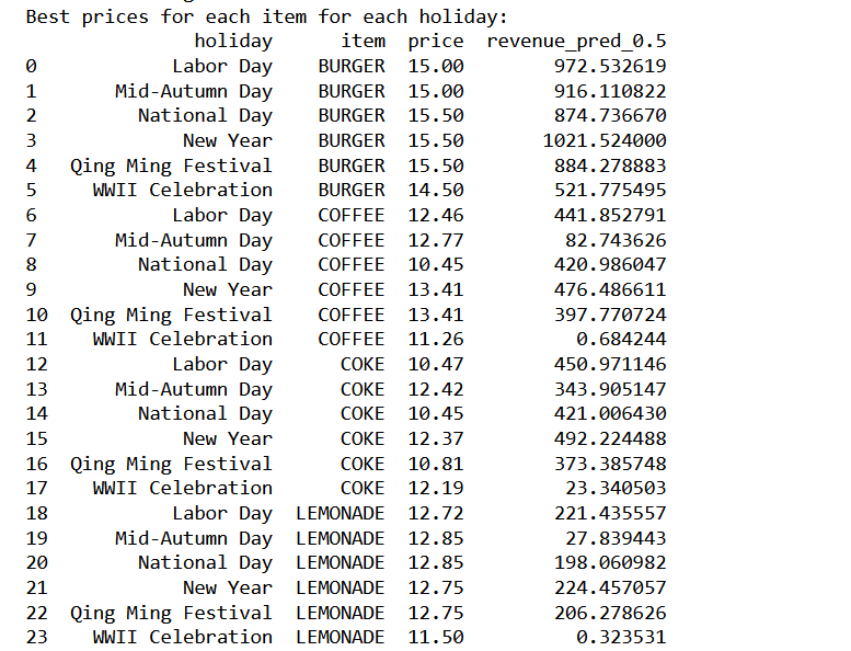
The analysis reveals the optimal pricing for various items tailored to specific holidays to maximize revenue. For instance, it suggests that the optimal price point for a burger on National Day is $15.50, while for WWII Celebration, it’s slightly lower at $14.50, reflecting a reduced demand on the latter holiday. In a similar manner, this approach allows us to ascertain the most profitable prices for different products across a range of holidays, taking into account the unique demand patterns observed on each occasion.

Conclusion:

In conclusion, this blog has explored the powerful intersection of machine learning and price optimization, demonstrating how advanced analytical models can significantly enhance pricing strategies. By utilizing techniques such as ExpectileGAM, businesses can analyze vast datasets to extract meaningful insights, allowing them to fine-tune their pricing for various products across different scenarios, including special events and holidays. This data-driven approach not only maximizes revenue but also ensures adaptability in a dynamic market, ultimately leading to smarter, more effective pricing decisions that benefit both the business and its customers.

References:

If you found this article interesting, your support by following below steps will help me spread the knowledge to others:

👏 Give the article 20 claps and hit the follow button

Follow me on LinkedIn

📚 Read more articles on Medium