Is F1-Score Really Better than Accuracy?

What’s the cost of being wrong (and the gain of being right) according to different metrics

If you google “What metric is better, accuracy or F1-score?” you will probably find an answer like:

“If your dataset is unbalanced, forget accuracy and go for F1-score.”

If you look for explanations, you will probably find a vague reference to the “different costs” associated with false negatives and false positives. But the sources do not state clearly which these costs are in the different metrics.

This is why I felt the need to write this article: to try and answer the following questions. What is the cost of false negatives and false positives in accuracy? And in F1-score? Is there a metric that allows us to assign custom values to such costs?

Starting from confusion

Both accuracy and F1-score can be calculated from the so-called confusion matrix. A confusion matrix is a square matrix comparing the labels predicted by our model with the true labels.

This is an example of a confusion matrix in the case of two labels: 0 (a.k.a. negatives) and 1 (a.k.a. positives). Note that, in this article, we will stick to binary classification, but everything we say can be generalized to the multiclass case.

Confusion matrix of a binary classifier. The elements of the matrix are true negatives (TN), false positives (FP), false negatives (FN), true positives (TP). [Image by Author]

As a result of the comparison, our observations may fall into these 4 cases:

True negatives (TN): our model correctly predicts 0.
False positives (FP): our model predicts 1, but the true label is 0.
False negatives (FN): our model predicts 0, but the true label is 1.
True positives (TP): our model correctly predicts 1.

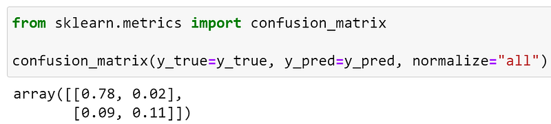
In Python, the simplest way to obtain the confusion matrix of a classifier is through Scikit-learn’s confusion_matrix. This function has two mandatory arguments: y_true (array of true values) and y_pred (array of predictions). In this case, I will also set the optional argument normalize="all" to get the relative count of observations, rather than the absolute count.

I have taken a dataset with 20% of positives and trained a model on it. This is the confusion matrix on the test set:

Computing confusion matrix with Scikit-learn. [Image by Author]

Here is a more friendly visualization of this outcome:

Let’s read it together:

True negatives (TN): 78% of the test set has been correctly labeled as 0.
False positives (FP): 2% of the test set has been mistakenly labeled as 1.
False negatives (FN): 9% of the test set has been mistakenly labeled as 0.
True positives (TP): 11% of the test set has been correctly labeled as 1.

The confusion matrix gives us all the information we may need about our classifier. However, we usually want a single metric that is able to summarize the performance of the model.

Two of the most popular metrics are accuracy and F1-score. Let’s see how they can be computed starting from the confusion matrix:

Accuracy: percentage of items classified correctly. It can be computed as the percentage of observations that are either true negatives or true positives. Having the confusion matrix, this is simply the sum of the elements on the principal diagonal, in this case: 78% + 11% = 89%.
F1-score: harmonic mean of precision and recall (of the positive class). This metric is a bit less intuitive than accuracy. Since F1 is based on precision and recall, let’s see how to compute these two metrics first. Precision is the percentage of predicted positives that are correctly classified, so precision = TP/(FP+TP) = 11%/(2%+11%) = 85%. Recall is the percentage of actual positives that are correctly classified, so recall = TP/(FN+TP) = 11%/(9%+11%) = 55%. Once we have precision and recall, F1 is the harmonic mean of these two quantities so: f1_score = (2*precision*recall)/(precision+recall) = (2*85%*55%)/(85%+55%) = 67%.

Now that we know what accuracy and F1-score are, let’s move on.

From one matrix to many matrices

You may not have noticed it, but the confusion matrix we have seen above comes from an arbitrary choice.

Indeed, the output of a binary classifier — in its rawest form — is not an array of labels, but rather an array of probabilities. For each observation, the classifier outputs the probability that it belongs to the positive class. To move from the probability to the label, we need to set a probability threshold.

Usually, the default threshold is set to 50%: any observation above 50% will be classified as 1, whereas any observation below that level will be classified as 0.

However, depending on the specific application, it may be preferable to use a different threshold. Let’s see how the confusion matrix would change based on the threshold that we set.

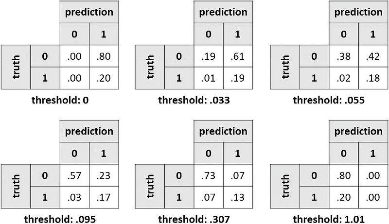
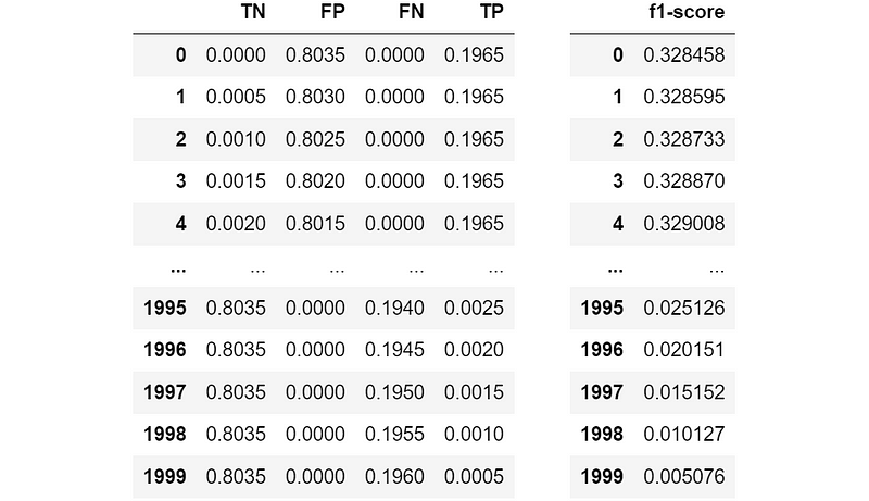
Confusion matrices of a binary classifier, depending on the probability threshold. [Image by Author]

Of course, as the threshold increases, we label fewer and fewer observations as positives: this is why the values under column “1” get smaller and smaller.

Here, we have seen 6 different thresholds as an example. However, the possible thresholds are often thousands. In these cases, it is more convenient to draw a plot. However, since the probability threshold doesn’t say much, I find it more convenient to put on the x-axis the % of observations that are predicted as positives, rather than the threshold itself.

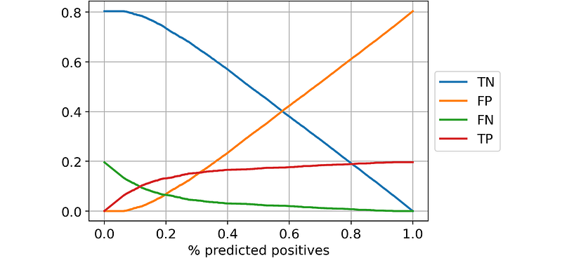
The four elements of the confusion matrix depending on the probability threshold (and so on the percentage of predicted positives). [Image by Author]

Also, for our purposes, it is probably more interesting to look directly at accuracy and F1-score rather than at the raw values of the confusion matrices.

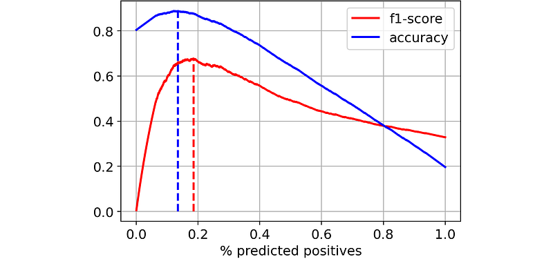
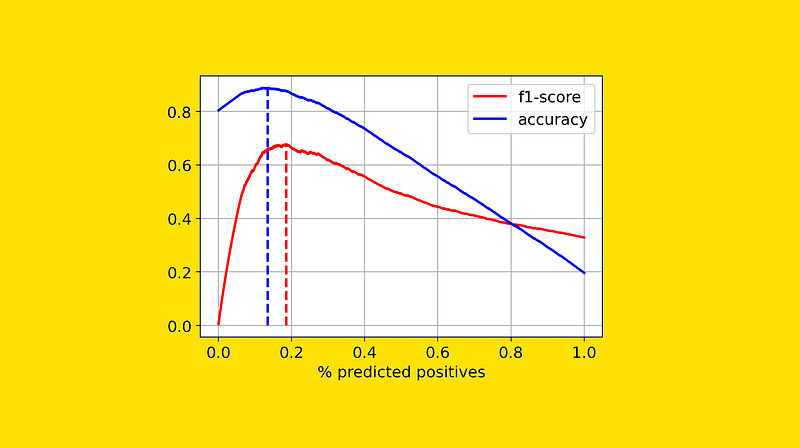
Accuracy and F1-score, depending on the probability threshold (and so on the percentage of predicted positives). [Image by Author]

Since both accuracy and F1-score are the-greater-the-better metrics, we would choose the threshold such that the corresponding metric is at its highest value. Thus, in the above plot, I have drawn a dashed line in correspondence with the maximum value of the respective metric.

As you can see, different metrics would lead us to choose different thresholds. In particular:

accuracy would lead us to choose a higher probability threshold, such that 14% of the observations are classified as positives.
F1-score would lead us to choose a smaller probability threshold, with more observations (19%) classified as positives.

So, which metric should we prefer?

The cost of wrong predictions

The common wisdom among practitioners is that F1-score must be preferred over accuracy, especially in unbalanced problems.

However, if you look for the reason why F1-score is supposedly superior to accuracy, you will find vague explanations. Many of them revolve around the “different costs” associated with false negatives and false positives. But they never clearly quantify these costs.

Moreover, focusing only on errors would give us a limited view of the problem. Indeed, if wrong predictions certainly carry a cost, then right predictions bring necessarily a profit.

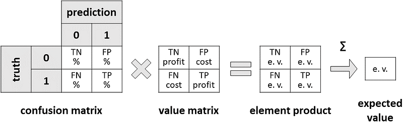
So, we should take into account not only the cost of false positives and false negatives but also the value of true positives and true negatives. From this idea, we can derive a new matrix — which I will call the “value matrix” — that assigns a (possibly economic) value to each element of the confusion matrix.

What’s the point of this matrix?

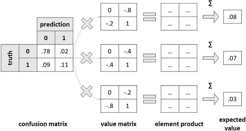
Well, since it assigns a value to each quantity of the confusion matrix, it is pretty natural to multiply these two matrices (element-wise) to obtain the expected value of any group (TN, FP, FN, TP).

This is an expected value because the confusion matrix contains the percentage of observations that belong to any group. Being a percentage, this can be interpreted as a probability. So, multiplying this probability by a (possibly economic) value gives us an expected value.

Summing the expected values of true negatives, false positives, false negatives and true positives gives us the expected value of the whole model.

The expected value of a binary classifier. The confusion matrix contains the frequency of each element. The value matrix contains the value (profit or loss) of each element. The element product of the two matrices yields the expected value of each component. Finally, summing them we obtain the overall expected value of the model. [Image by Author]

The decomposition into confusion matrix and value matrix is very intuitive also for non-technical stakeholders. After all, everyone can understand percentages and dollars!

At this point, we are ready to answer the initial question: what are the value matrices of accuracy and F1-score?

Finding the value matrix of accuracy

We have already seen that accuracy simply sums the values on the principal diagonal of the confusion matrix. Thus, it is straightforward to prove that the value matrix of accuracy is the identity matrix.

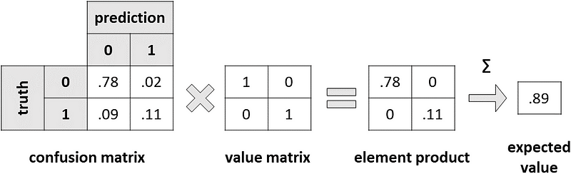
Accuracy as the expected value of a classifier. [Image by Author]

The shortcoming of accuracy should be immediately apparent: it is equivalent to assuming that we gain 1 in the case of right predictions (true negatives or true positives) and we don’t lose anything in case of wrong predictions. This assumption is at the very least unlikely for most use cases.

Finding the value matrix of F1-score

So what are the values associated with right/wrong answers in F1-score?

In practice, we would like to find out which elements of the value matrix will give us the resulting F1-score. This corresponds to filling in the question marks in the following figure:

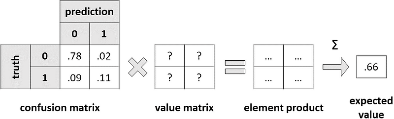
F1-score as the expected value of a classifier. [Image by Author]

Unfortunately for us, the answer is not as simple as it was for accuracy. In fact, in this case, there is no closed-form solution. However, we can exploit the information we have extracted from the different thresholds:

F1-score for different confusion matrices (based on different probability thresholds). [Image by Author]

We can use true negatives, false positives, false negatives and true positives as independent variables and the resulting F1-score as the dependent variable. It’s enough to fit a linear regression to get an estimate of the resulting coefficients (i.e. the numbers to fill our value matrix).

In this case, these are the values that we get:

Value matrix (estimated through linear regression) for F1-score. [Image by Author]

It is clear from here that F1-score puts more stress on positive observations (whether they are classified as 0 or 1).

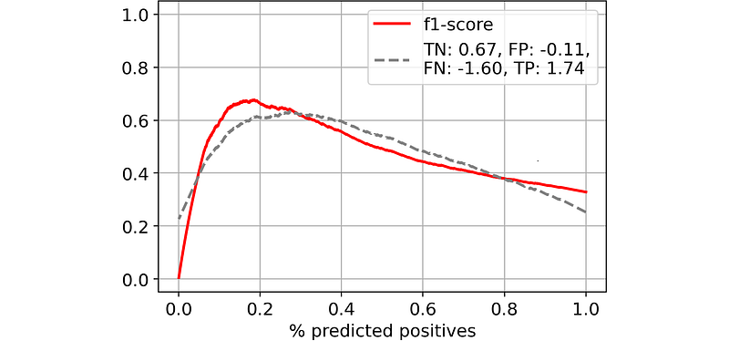
Note that this is an approximate solution! Differently from accuracy, an exact solution for the value matrix does not exist here. If you are curious, this is our result (dashed line) compared to the actual curve of F1-score.

Actual F1-score vs. our estimated curve. [Image by Author]

Beyond accuracy and F1-score

We have seen the value matrices of accuracy and F1-score. The former is arbitrary and the latter cannot be even calculated directly (it will be an approximate solution anyway).

So, why not just set our custom value matrix?

In fact, depending on your use case, it should be relatively easy to figure out how much a wrong (right) prediction costs (is worth) to you.

Let’s make an example. You want to predict which customers are more likely to churn. You know that a customer is worth on average $10 per month. In order to prevent customers to leave the company, you want to propose to them a discount that cuts your profit by $2 per customer (let’s here assume that the discount will be accepted by everyone).

So your value matrix will be the following:

Value matrix for churn example. [Image by Author]

Why is that?

True Negatives: $0. Your prediction task will not affect them, so the value is 0.
False Positives: -$2. You are giving them a discount, but they wouldn’t churn anyway, so you are cutting your profit by $2 for nothing.
False Negatives: $0. Your prediction task will not affect them, so the value is 0.
True Positives: +$8. You correctly predicted that they would churn, so you save $8 ($10 minus $2 due to your action).

The point is that the characteristics of the value matrix depend entirely on your specific use case.

For instance, let’s set some example value matrices, and see how the respective expected value would change.

Some examples of how the expected value of a classifier changes according to the value matrix. [Image by Author]

We can repeat this process for all the possible thresholds:

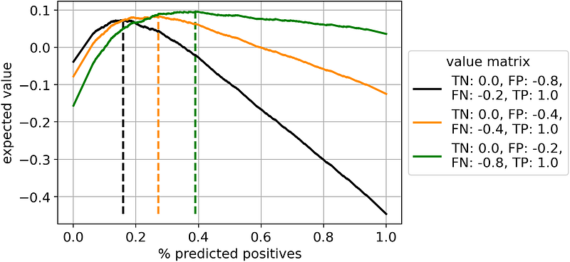
The expected value of a classifier, depending on the value associated with right/wrong predictions. [Image by Author]

Differently from accuracy and F1-scores, these custom KPIs may assume negative values. This makes a lot of sense! In fact, in the real world, there are scenarios in which your classifier can make you lose money. For sure, you want to be aware of that possibility in advance, and this custom metric allows you to do that.

It’s interesting to observe the behavior of the three curves. Other things being equal, a higher cost of false negatives and a lower cost of false positives (i.e. moving from the black to the green line) incentivizes us to predict more observations as positives (i.e. from 16% to 39%). It’s intuitive: a high cost for false negatives is an incentive to classify fewer observations as negatives, and vice-versa.

In general, using a custom value matrix allows you to place yourself in the perfect spot in the precision/recall trade-off.

Conclusions

In this article, we have compared accuracy and F1-score, based on the different costs that they attribute to errors.

Accuracy is a bit naive since it attributes a value of 1 to correct predictions and a null cost to errors. On the other hand, F1-score is more like a black box: you will always need to reverse-engineer it to get its value matrix (and, in any case, it will be an approximate solution).

My advice is to use a custom value matrix, depending on your specific application. Once you have set the value matrix, you can multiply it by your confusion matrix and get the expected value of your classifier. This is the only way to get an idea of the actual economic impact of using your classifier out there in the real world.

Thank you for reading!

If you find my work useful, you can subscribe to get an email every time that I publish a new article (usually once a month).

If you want to support my work, you can buy me a coffee.

If you’d like, add me on Linkedin!