
Investment: Efficient Frontier and Capital Market Line Explained
The note below is for review purposes and is not intended to be used as initial study materials. I am trying to summarize the key points using as few mathematics formulas as possible while capturing the main philosophy of the models.
Efficient Frontier
Judging by its name, modern portfolio theory (MPT) is about finding the optimal portfolio. Efficient Frontier is part of the MPT.
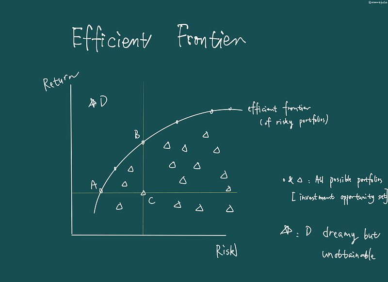
We first plot all possible risky portfolios onto the graph, according to their risk-return inputs. This step is also referred to as identifying the investment opportunity set.
Basically, we are looking to answer this question: What’s available out there?
(Markowitz) efficient frontier links a series of these portfolios and answering the question: What’s the “best” (most efficient) available out there? Efficient here means offering the highest possible returns for any level of risk.
What does possible mean here? Above this curve, returns are too good to be true. In other words, portfolios above the efficient frontier have unobtainable returns given the level of risks they entail. Looking at point D, dreamy but unobtainable.
The assumptions of MPT determine the “highest” part of the definition.
Assumptions:
- Investors are risk-averse (requires a higher return to compensate for higher risks.)
- For any level of risk (low or high), investors would want the highest possible returns. (Higher returns are preferred to lower returns at any level of risk.) [Help choosing portfolios vertically: B is preferred to C.]
- Similarly, at any level of returns, investors prefer the lowest possible level of risks. (Lower risks are preferred to higher risks.) [Help choosing portfolios horizontally: A is preferred to C.]
So now, we have selected a subset of risky portfolios out of all possible portfolios.
The quest does not stop here, though. There are numerous portfolios on the efficient frontier. What’s next? We introduce the capital market line to help narrow down “the one.”
Capital Allocation Line (CAL) and Capital Market Line (CML)
When we were identifying efficient frontier, we were only looking at all risky portfolios. Besides securities, risk-free assets (government debt) are also investment opportunities.
Once we introduce risk-free assets, we can leverage the capital allocation line (CAL) to choose an allocation including risk-free and risky assets. Risk-free return is given to us; the question is about the weight that should be allocated to the risk-free asset. As for the risky portfolio part, there are two questions: which portfolio and what weight?
Which risky portfolio to choose? The candidates are all included in the efficient frontier. We can draw many CALs that have the same intercept (risk-free return) and different slopes. We want the one with the largest slope (the steepest) possible, later called the Capital Market Line (CML).
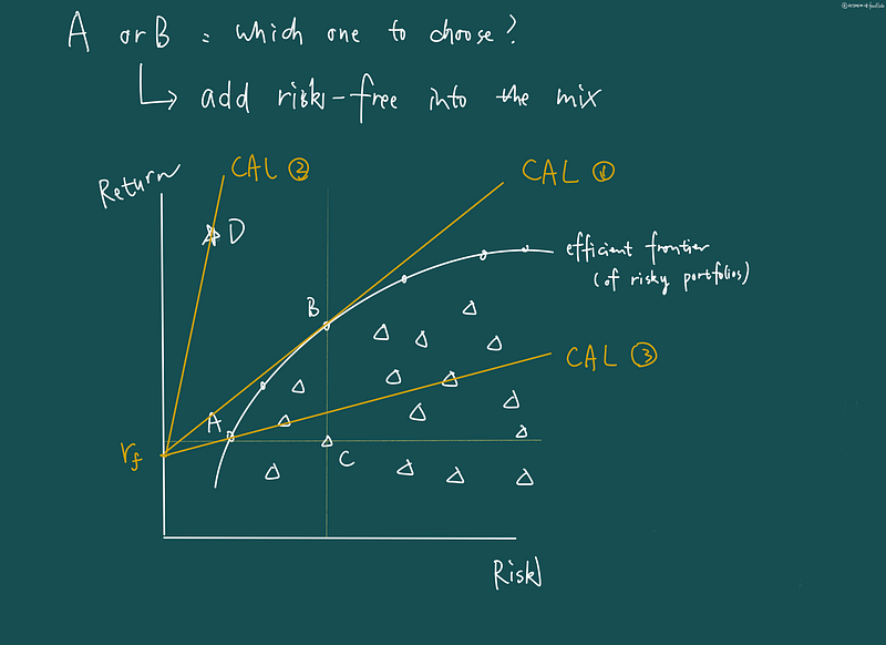
So in our illustration, CAL №1 is the CML, and Point B is the optimal risky portfolio. CAL №2 is too dreamy to be true. Why is CAL №1 better than CAL №3? For any given level of risk, №1 offers higher returns.
Once we introduce a risk-free rate, CML replaces the “old” efficient frontier and becomes the NEW efficient frontier. Each point along CML depicts an efficient allocation between risk-free and risky assets.
At point B, the tangency point, the investor is only invested in risky portfolios (remember, B is also on the “old” efficient frontier, which only discusses risky portfolios). To the left of B (risk is lower), the investor allocates some to risky portfolios and some to risk-free assets. At the intercept, all is allocated to risk-free assets. To the right of B, the higher return is generated using borrowed funds to invest in risky portfolios.
Final notes on CML
- CML talks about returns and risks for portfolios, not individual security.
- Formula:
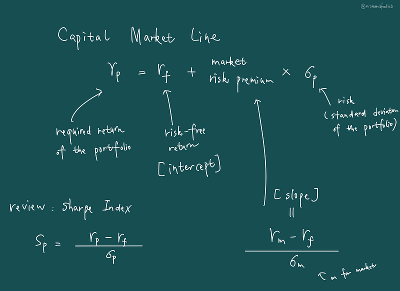
- Risk is measured using standard deviation.
- The slope of CML is very similar to Sharpe Index. In fact, it’s a special case of the Sharpe Index. The slope of CML is when we measure the risk premiums of the whole market instead of a specific portfolio (Sharpe). So you now remember that Sharpe Index also uses stand deviation to measure risk.
Do you have any other questions on this topic? If so, please leave a comment and let me know!