Inverse Projection Transformation

Depth and Inverse Projection

When an image of a scene is captured by a camera, we lose depth information as objects and points in 3D space are mapped onto a 2D image plane. This is also known as a projective transformation, in which points in the world are converted to pixels on a 2d plane.

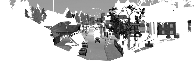
However, what if we want to do the inverse? That is, we want to recover and reconstruct the scene given only 2D image. To do that, we would need to know the depth or Z-component of each corresponding pixels. Depth can be represented as an image as shown in fig 2 (centre). With brighter intensity denoting point further away.

Understanding depth perception is essential in many computer vision applications. For example, able to measure depth for an autonomous vehicle allows for better decision making as the agent is fully aware of the separation distances between other vehicles and pedestrians.

Difficulty reasoning in perspective view

Consider fig 2 above, given only the RGB image. It is hard to tell what is the absolute distance between the 2 cars on the left lane. Also, I most certainly find it difficult to perceive whether the trees on the left are indeed very near or it is extremely far from the house. The above phenomenon is a consequence of perspective projection, which requires us to rely on various cues to come up with a good estimate of the distance. I discussed some of the issues with perspectivity in this post which might interest you:)

However, if we were to reproject it back to 3d with the aid of a depth map (fig 2. right), we could accurately position the trees and perceive that they are actually distanced away from the building. Yes, we are really bad at figuring the relative depth when an object is occluded behind another object. The main takeaway from this is looking at images alone, it is hard to discern depth.

The problem of estimating depth is an on-going research and has well progressed over the years. Many techniques have been developed and the most successful methods come from determining depth using stereo vision[1]. And in recent years, depth estimation using deep learning has shown incredible performance [2], [3].

In this article, we will take a tour and understand the mathematics and concepts of performing back-projection from 2D pixels coordinate to 3D points. I will then go through a simple example in Python to show the projection in action. Code is available here. We will assume that a depth map is provided to perform the 3D reconstruction. The concepts that we will go through are camera calibration parameters, projective transformation using intrinsic and its inverse, coordinate transformation between frames.

Central Projection of Pinhole Camera Model

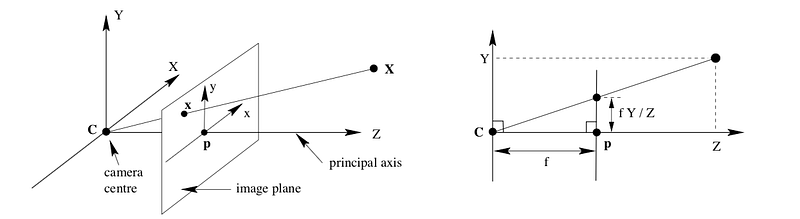
First and foremost, understanding the geometrical model of the camera projection serves as the core idea. What we are ultimately interested in is the depth, parameter Z. Here, we consider the simplest pinhole camera model with no skew or distortion factor.

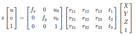
3D points are mapped to the image plane (u, v) = f(X, Y, Z). The complete mathematical model that describes this transformation can be written as p = K[R|t] * P.

where

• p is the projected point on the image plane
• K is the camera intrinsics matrix
• [R|t] is the extrinsic parameters describing the relative transformation of the point in the world frame to the camera frame
• P, [X, Y, Z, 1] represents the 3D point expressed in a predefined world coordinate system in Euclidean space
• Aspect ratio scaling, s: controls how pixels are scaled in the x and y direction as focal length changes

Intrinsic parameter matrix

The matrix K is responsible for projecting 3D points to the image plane. To do that, the following quantities must be defined as

• Focal length (fx, fy): measure the position of the image plane wrt to the camera centre.
• Principal point (u0, v0): The optical centre of the image plane
• Skew factor: The misalignment from a square pixel if the image plane axes are not perpendicular. In our example, this is set to zero.

The most common way of solving all the parameters is using the checkerboard method. Where several 2D-3D correspondences are obtained through matching and solving the unknown parameters by means of PnP, Direct Linear Transform or RANSAC to improve robustness.

With all the unknowns determine, we can finally proceed to recover the 3D points (X, Y, Z) by applying the inverse.

Backprojection

Consider the equation in Fig 4. Suppose (X, Y, Z, 1) is in the camera coordinate frame. i.e. we do not need to consider the extrinsic matrix [R|t]. Expanding the equation would give as

The 3D points can be recovered with Z given by the depth map and solving for X and Y. We can then further transform the points back to the world frame if needed.

Inverse projection example

Let's go through a simple example to digest the concepts. We will use the RGB and depth image as shown in figure 1. Pictures are acquired from a camera mounted on a car in a simulator, CARLA. The depth map is stored as float32 and encodes up to a maximum of 1000m for depth values at infinity.

Intrinsic Parameters from Field of View

Instead of determining the intrinsic parameters using checkerboard, one can calculate the focal lengths and optical centre for the pinhole camera model. The information needed is the imaging sensor height and width in pixels and the effective field of view in the vertical and horizontal direction. Camera manufacturer usually provides those. In our example, we will use +-45 degrees both in the vertical and horizontal direction. We will set the scale factor to 1.

Referring to fig 3, the focal lengths (fx, fy) and the principal point (u0, v0) can be determined using simple trigonometry. I leave it up to you to derive it as an exercise or you can look it up in the code!

Now, we can compute the inverse as follows

• Obtain the intrinsic camera parameters, K
• Find the inverse of K
• Apply equation in fig 5 with Z as depth from a depth map.

# Using Linear Algebra
cam_coords = K_inv @ pixel_coords * depth.flatten()

A slower but more intuitive way of writing step 3 is

cam_points = np.zeros((img_h * img_w, 3))
i = 0
# Loop through each pixel in the image
for v in range(height):
    for u in range(width):
        # Apply equation in fig 5
        x = (u - u0) * depth[v, u] / fx
        y = (v - v0) * depth[v, u] / fy
        z = depth[v, u]
        cam_points[i] = (x, y, z)
        i += 1

You will get the same results!

Conclusion

There we have it, I have gone through the basic concepts required to do a back-projection.

Back projecting to 3D forms the basis of 3D scene reconstruction via Structure form Motion where several images are captured from a moving camera, along with its depth known or computed. Thereafter, matching and stitching together to get a complete understanding of the scene structure.

Orthographic Projection: Top View (Optional)

With the points represented in 3D, one interesting application is to project it to a top-down view of the scene. This is usually a useful representation for mobile robots as the distances between obstacles are preserved. Furthermore, it is easy to interpret and utilize to perform path planning and navigation task. For this, we need to know the coordinate system in which the points references.

We will use the right-hand coordinate system as defined below

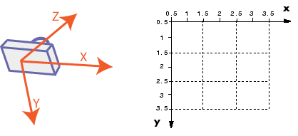
For this simple example, which plane do you think the points should be projected?

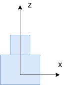
If your guess is on the plane y= 0, you are right as y represent height as defined by the camera coordinate system. We simply collapse the y component in the projection matrix.

Looking at the figure below, you can easily measure the separation distances between all vehicles and objects.

Reference

[1] Hirschmuller, H. (2005). Accurate and Efficient Stereo Processing by Semi Global Matching and Mutual Information. CVPR

[2] Tinghui Zhou, Matthew Brown, Noah Snavely, and David Lowe. Unsupervised learning of depth and ego-motion from video. In CVPR, 2017

[3] Clement Godard, Oisin Mac Aodha, and Gabriel J Brostow. Unsupervised monocular depth estimation with left-right consistency. In CVPR, 2017.