Introduction to Machine Learning: Regression

Introduction

This article covers regression analysis, which is fundamental to many applications of machine learning and throughout scientific disciplines. We will walk through some of the concepts and then dig into some regression examples using financial data from AlphaWave Data.

Jupyter Notebooks are available on Google Colab and Github. For this analysis, we use several Python-based scientific computing technologies listed below.

#Import Libraries
import math
import time
import requests
import numpy as np
import pandas as pd
from scipy import stats
import plotly.express as px
import plotly.graph_objects as go
from datetime import datetime, timedelta
from sklearn.linear_model import LinearRegression

Regression: a branch of supervised learning

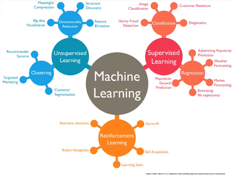
In the context of machine learning, regression is a branch of supervised learning algorithms. Supervised learning requires labeled training data as well as matched sets of observed inputs (X’s, or features) and the associated output (Y, or target). It can be divided into two categories: regression and classification. If the target variable to be predicted is continuous, then the task is one of regression. If the target variable is categorical or ordinal (e.g., determining a firm’s rating), then it is a classification problem.

Other machine learning approaches outside the supervised learning bubble do make use of regression as part of their algorithm also. For example, clustering is often done using logistic regression.

In doing a regression, we are trying to fit a model to the data that was observed so that we can use this model to predict the future. Data is usually messy and noisy. Regression is a technique to quantify the substance of what is observed in the world into a simplified model. In simple linear regression, we find the best fitting line through the observed points.

We can write an equation for a line as: Y= mX + b. Y: dependent variable, also known as response variable or outcome variable X: independent variable, also known as the explanatory variable or predictor variable

Y is a dependent variable and X is the independent variable. We observe the values of X and Y and then use these to estimate the slope m and the intercept b. When regressing the returns of IBM against the returns of SPY (an ETF that is designed to track the S&P 500 stock market index), the slope m of the regression line would be the market Beta for IBM and the intercept b would be the alpha.

When a linear regression is discussed as being in the form of a parametric model, it means all its information is represented within its parameters. In the case of this line, all of the information of the model can be captured by these two parameters slope and intercept. All you need to define a line is m and b. In the parlance of machine learning, this act of estimating the parameters based on some observable data is the process of training the model.

The simplest linear regression approach is ordinary least squares (OLS). In regression, we are trying to minimize something. In OLS, we are drawing the prediction line to minimize the sum of the squares of the difference between the line and the data. So the further away a point is from our prediction line, it penalizes the model by the square of that discrepancy.

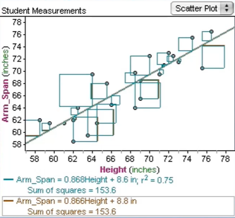
It’s important to quantify how good of a regression fit you have. One of these measures is the mean squared error, which is the average size of each of the squares in the graph above. The most commonly used goodness of fit measure is the R squared, which is essentially a standardized version of the squared deviation that will always be a number between 0 and 1.

One other notable example of regression in finance is the Fama-French three-factor model. Instead of having just one X variable, we have three Xs or three explanatory variables. In the case of Fama-French, they are expressing the return of stocks as dependent on the return of the market, the outperformance of small-cap stocks over large-cap stocks, and the outperformance of high-value stocks over low-value stocks. Using these observed factor returns, which Fama and French define, they estimate these three beta sensitivities to explain the return of stocks in the market.

Linear Regression Examples

Single Variable:

Market Model Regression: y = α + β X

Multiple Variable:

Fama-French: y = α + βMKT*RMKT + βSMB*RSMB + βHML*RHML
Multi-Factor Model: y = α + β1*X1 + β2*X2 + β3*X3

In a fundamental multi-factor model’s observed factor returns, you are doing a multivariate regression to estimate all factor betas like sector returns, momentum, and low volatility stock performance.

Linear regression maps a continuous variable X to continuous variable Y. But when Y, our response variable, is discrete meaning it can only be a 0 or 1 or a finite number of categorical values, then we can do logistic regression.

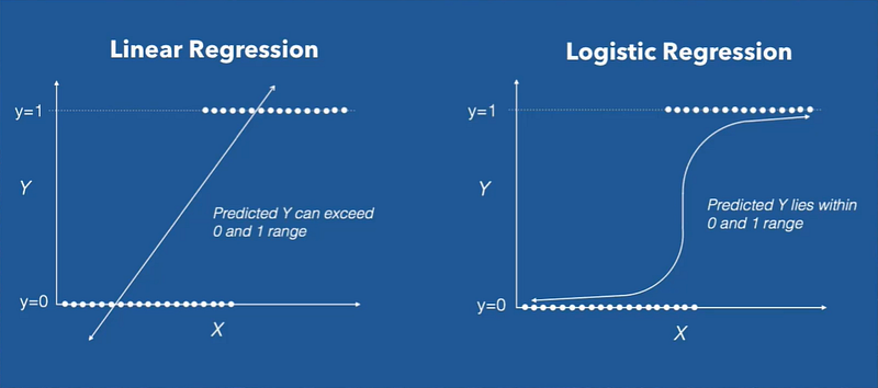
Rather than modeling the response variable directly, logistic regression models the probability that Y belongs to a particular category. This means you are trying to maximize a likelihood. As a result, logistic regression is often used in Classification algorithms. For example, will a company default on its debt?

Terminology

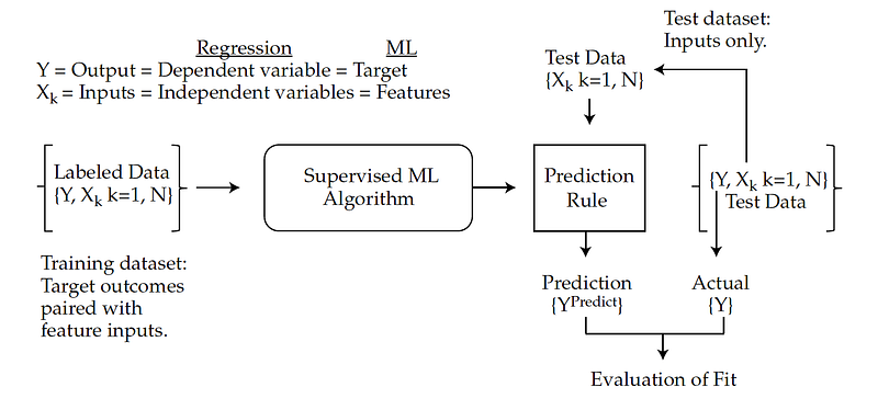
The terminology used with ML algorithms differs from that used in the regression. In supervised machine learning, the dependent variable (Y) is the target and the independent variables (X’s) are known as features. The labeled data (training data set) is used to train the supervised ML algorithm to infer a pattern-based prediction rule. The fit of the ML model is evaluated using labeled test data in which the predicted targets (Y Predict) are compared to the actual targets (Y Actual).

Below provides a visual of the supervised learning model training process and a translation between regression and ML terminologies.

Example 1: Regression of returns of IBM against SPY

As our first example, we are going to regress the daily returns of IBM against the returns of SPY. We can use the 1 Year Historical Daily Prices endpoint from the AlphaWave Data Stock Prices API to pull in the one-year historical prices. With these prices, we can produce a scatter plot with IBM returns on the Y-axis and SPY returns on the X-axis to get a sense of what this data looks like.

#fetch daily return data for IBM and SPY ETF
stock_tickers = ['IBM','SPY']

To call this API with Python, you can choose one of the supported Python code snippets provided in the API console. The following is an example of how to invoke the API with Python Requests. You will need to insert your own x-RapidAPI-host and x-RapidAPI-key information in the code block below.

#fetch 1 year daily return data
url = "https://stock-prices2.p.rapidapi.com/api/v1/resources/stock-prices/1y"

headers = {
    'x-rapidapi-host': "YOUR_X-RAPIDAPI-HOST_WILL_COPY_DIRECTLY_FROM_RAPIDAPI_PYTHON_CODE_SNIPPETS",
    'x-rapidapi-key': "YOUR_X-RAPIDAPI-KEY_WILL_COPY_DIRECTLY_FROM_RAPIDAPI_PYTHON_CODE_SNIPPETS"
    }

stock_frames = []

for ticker in stock_tickers:
    querystring = {"ticker":ticker}
    stock_daily_return_response = requests.request("GET", url, headers=headers, params=querystring)

# Create Stock Prices DataFrame
    stock_daily_return_df = pd.DataFrame.from_dict(stock_daily_return_response.json())
    stock_daily_return_df = stock_daily_return_df.transpose()
    stock_daily_return_df = stock_daily_return_df.rename(columns={'Close':ticker + ' Close'})
    stock_daily_return_df = stock_daily_return_df[{ticker + ' Close'}]
    stock_frames.append(stock_daily_return_df)

combined_stock_return_df = pd.concat(stock_frames, axis=1, join="inner")
pct_change_combined_stock_df = combined_stock_return_df.pct_change()
pct_change_combined_stock_df = pct_change_combined_stock_df.dropna()
pct_change_combined_stock_df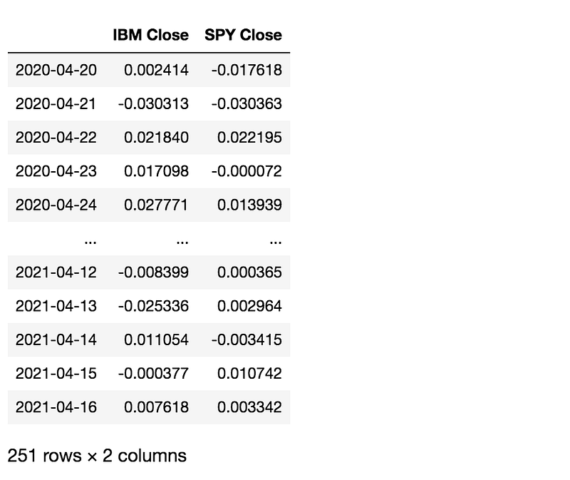

Plot daily return of IBM against the daily return of SPY:

fig = px.scatter(
    pct_change_combined_stock_df, x=stock_tickers[1] + ' Close', y=stock_tickers[0] + ' Close',
    trendline='ols', trendline_color_override='red'
)
fig.update_layout(template='plotly_dark', xaxis_title=stock_tickers[1] + " Daily Return", yaxis_title=stock_tickers[0] + " Daily Return",yaxis_tickformat = '.2%',xaxis_tickformat = '.2%')
fig.show()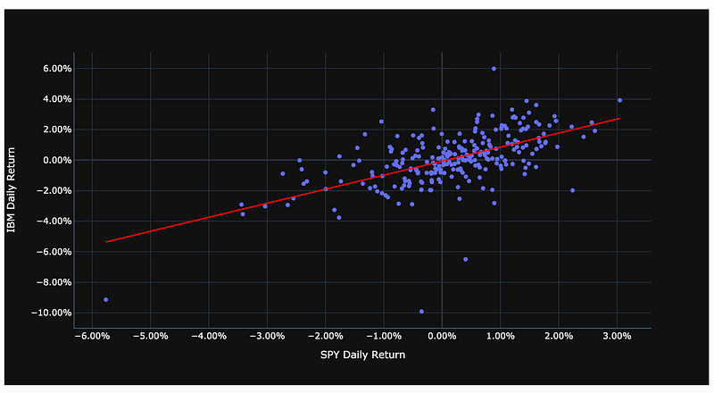

We can now use the SciPy library for OLS. Using the stats.lineregress function in SciPy, we can produce the slope, intercept, r-value, p-value, and standard error parameters.

SciPy Linear Regression: https://docs.scipy.org/doc/scipy/reference/generated/scipy.stats.linregress.html

slope, intercept, r_value, p_value, std_err = stats.linregress(x=pct_change_combined_stock_df[stock_tickers[1]+' Close'],
                                                               y=pct_change_combined_stock_df[stock_tickers[0]+' Close'])

OLS regression coefficients:

slope, intercept, r_value, p_value, std_err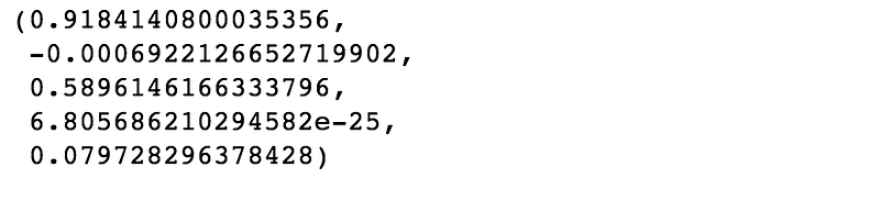

R Squared:

r_value*r_value

Using the Plotly visualization library, we can graph the scatter plot of daily returns and the OLS regression line from scratch with the code below.

#initialize figure
fig = go.Figure()
fig.add_trace(go.Scatter(x=pct_change_combined_stock_df[stock_tickers[1]+' Close'], \
                         y=pct_change_combined_stock_df[stock_tickers[0]+' Close'],
                    mode='markers', name='Daily return',))

#construct regression line from its coordinates from the scipy regression coefficients
line_x = [pct_change_combined_stock_df[stock_tickers[1]+' Close'].min(),  \
          pct_change_combined_stock_df[stock_tickers[1]+' Close'].max()]
line_y = [line_x[0]*slope+intercept,  line_x[1]*slope+intercept]

#add regression line to this plot
fig.add_trace(go.Scatter(x=line_x,y=line_y,name='OLS regression line', mode='lines'))

#show the figure
fig.update_layout(template='plotly_dark', xaxis_title=stock_tickers[1] + " Daily Return", yaxis_title=stock_tickers[0] + " Daily Return", yaxis_tickformat = '.2%',xaxis_tickformat = '.2%')
fig.show()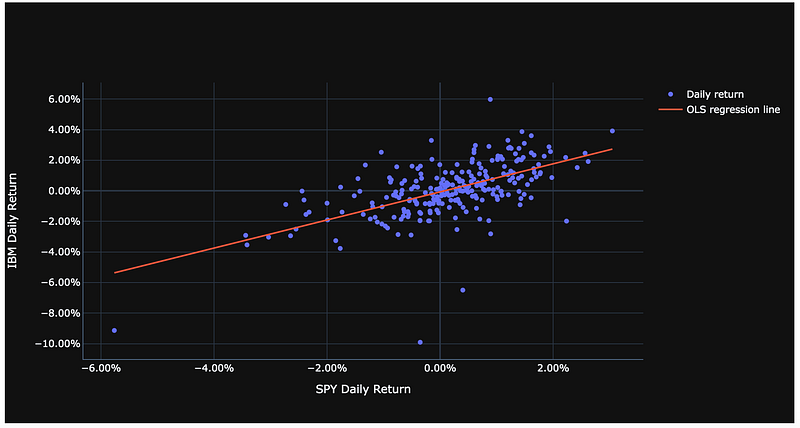

However, Plotly has made it easy to automatically plot our data and the OLS regression line all at once using the code below because plotting the regression line is often used.

Example: Plotly — ML Regression in Python

fig = px.scatter(
    pct_change_combined_stock_df, x=stock_tickers[1] + ' Close', y=stock_tickers[0] + ' Close',
    trendline='ols', trendline_color_override='red'
)
fig.update_layout(template='plotly_dark', xaxis_title=stock_tickers[1] + " Daily Return", yaxis_title=stock_tickers[0] + " Daily Return",yaxis_tickformat = '.2%',xaxis_tickformat = '.2%')
fig.show()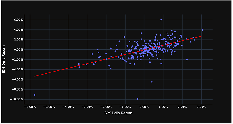

The IBM versus SPY regression example below is a regression using math and Numpy only instead of SciPy.

Website reference:

https://towardsdatascience.com/linear-regression-from-scratch-cd0dee067f72

How To Implement Simple Linear Regression From Scratch With Python - Machine Learning Mastery

Linear regression is a prediction method that is more than 200 years old. Simple linear regression is a great first…

machinelearningmastery.com

pct_change_combined_stock_df.tail()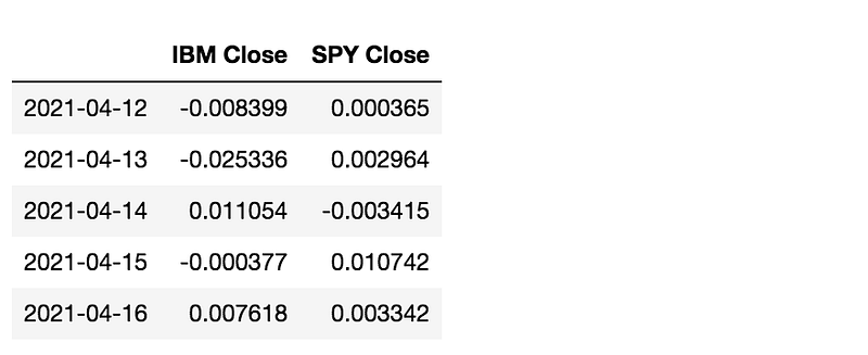

X = pct_change_combined_stock_df[stock_tickers[1]+' Close'].values
y = pct_change_combined_stock_df[stock_tickers[0]+' Close'].values

#Calculate mean of dependent variable (IBM) returns and independendent variable (SPY) returns
x_mean = np.mean(X)
y_mean = np.mean(y)

#total N
n = len(X)

#calculate the coefficients by calculating the squared distance
numerator = 0
denominator = 0

for i in range(n):
    numerator += (X[i] - x_mean) * (y[i] - y_mean)
    denominator += (X[i] - x_mean) ** 2
    
slope = numerator / denominator
slope

intercept = y_mean - (slope * x_mean)
intercept

Calculate the R Squared:

sumofsquares = 0 
sumofresiduals = 0

#sum total squares over some of total residuals
for i in range(n):
    predicted_y = intercept + slope * X[i]
    sumofsquares += (y[i] - y_mean) ** 2
    sumofresiduals += (y[i] - predicted_y) ** 2
    
r2_score = 1 - (sumofresiduals/sumofsquares)
r2_score

Example 2: Bitcoin return vs SPY

In our second example, we regress the two-year weekly returns of Bitcoin against SPY. This regression will explore some of the reasons why regression does not always work so well, like when overfitting the data.

We will first use the 2 Year Historical Daily Prices endpoint from the AlphaWave Data Stock Prices API to pull in the two-year daily historical prices for Bitcoin and SPY. We then convert the price data to daily returns.

#fetch daily return data for Bitcoin and SPY ETF
bitcoin_tickers = ['BTC-USD','SPY']

#fetch 2 year daily return data
url = "https://stock-prices2.p.rapidapi.com/api/v1/resources/stock-prices/2y"

headers = {
    'x-rapidapi-host': "YOUR_X-RAPIDAPI-HOST_WILL_COPY_DIRECTLY_FROM_RAPIDAPI_PYTHON_CODE_SNIPPETS",
    'x-rapidapi-key': "YOUR_X-RAPIDAPI-KEY_WILL_COPY_DIRECTLY_FROM_RAPIDAPI_PYTHON_CODE_SNIPPETS"
    }

bitcoin_frames = []

for ticker in bitcoin_tickers:
    querystring = {"ticker":ticker}
    bitcoin_daily_return_response = requests.request("GET", url, headers=headers, params=querystring)

# Create Stock Prices DataFrame
    bitcoin_daily_return_df = pd.DataFrame.from_dict(bitcoin_daily_return_response.json())
    bitcoin_daily_return_df = bitcoin_daily_return_df.transpose()
    bitcoin_daily_return_df = bitcoin_daily_return_df.rename(columns={'Close':ticker + ' Close'})
    bitcoin_daily_return_df = bitcoin_daily_return_df[{ticker + ' Close'}]
    bitcoin_frames.append(bitcoin_daily_return_df)

combined_bitcoin_price_df = pd.concat(bitcoin_frames, axis=1, join="inner")
pct_change_combined_bitcoin_df = combined_bitcoin_price_df.pct_change()
pct_change_combined_bitcoin_df = pct_change_combined_bitcoin_df.dropna()
pct_change_combined_bitcoin_df.index =  pd.to_datetime(pct_change_combined_bitcoin_df.index)
pct_change_combined_bitcoin_df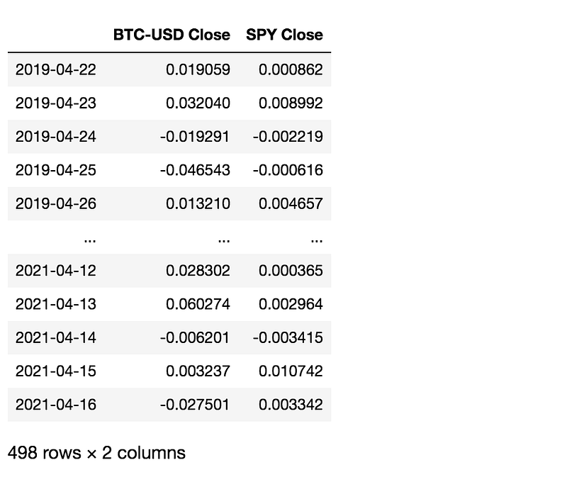

Because we currently have two years of daily returns for Bitcoin and SPY, we will use the code below to convert this data into the desired weekly returns. We then produce a scatter plot with Bitcoin returns on the Y-axis and SPY returns on the X-axis to get a sense of what this data looks like.

#convert daily return data into weekly return data
combined_bitcoin_price_df = combined_bitcoin_price_df.dropna()
weekly_pct_change_combined_bitcoin_df = combined_bitcoin_price_df.pct_change(periods=5)
weekly_pct_change_combined_bitcoin_df = weekly_pct_change_combined_bitcoin_df.iloc[::5, :].dropna()
weekly_pct_change_combined_bitcoin_df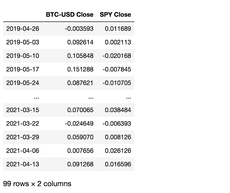

fig = px.scatter(
    weekly_pct_change_combined_bitcoin_df, x=bitcoin_tickers[1] + ' Close', y=bitcoin_tickers[0] + ' Close', opacity=0.65, 
    trendline='ols', trendline_color_override='red', title='2 year weekly BTC vs SPY' 
)
fig.update_layout(template='plotly_dark', xaxis_title=bitcoin_tickers[1] + " Weekly Return", yaxis_title=bitcoin_tickers[0] + " Weekly Return", yaxis_tickformat = '.1%',xaxis_tickformat = '.1%')
fig.show()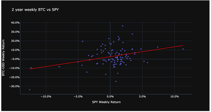

The Bitcoin regression is not a good fit, which can be seen with an R squared of approximately 0.10.

We can attempt to improve the model fit with the Bitcoin data, but we risk overfitting in doing so. To test if a better model fit can be achieved, we can work with Scikit-learn and use the PolynomialFeatures.

Scikit-learn Linear Regression: https://scikit-learn.org/stable/modules/generated/sklearn.linear_model.LinearRegression.html

Scikit-learn Polynomial Features: https://scikit-learn.org/stable/modules/generated/sklearn.preprocessing.PolynomialFeatures.html

Overfitting means training a model to such a degree of specificity to the training data that the model begins to incorporate noise coming from quirks or spurious correlations; it mistakes randomness for patterns and relationships. The algorithm may have memorized the data, rather than learned from it, so it has perfect hindsight but no foresight. The main contributors to overfitting are thus high noise levels in the data and too much complexity in the model.

We use a polynomial linear regression with a degree of 9 to see if we can get a better fit with the Bitcoin data.

from sklearn.preprocessing import PolynomialFeatures
from sklearn.pipeline import make_pipeline
from sklearn.linear_model import LinearRegression

#Fetch weekly return data of BTC and SPY  (This is our training data set)
df_X = weekly_pct_change_combined_bitcoin_df[{bitcoin_tickers[1] + ' Close'}]
df_y = weekly_pct_change_combined_bitcoin_df[{bitcoin_tickers[0] + ' Close'}]

#Fit training data to a polynomial regression model using sklearn.preprocessing and sklearn.pipeline
degree=9
polyreg=make_pipeline(PolynomialFeatures(degree),LinearRegression())
polyreg.fit(df_X,df_y)

#Using the predicted model, get the projected values over the space of X
X_seq = np.linspace(df_X.min(),df_X.max(),300).reshape(-1,1)
pred_y = polyreg.predict(X_seq)
l_pred_y = list(pred_y.reshape(-1,len(pred_y))[0])
l_X_seq = list(X_seq.reshape(-1,len(X_seq))[0])
df_scat = pd.DataFrame(data={'x':l_X_seq,'y':l_pred_y})

#Plot the original observations (BTC weekly returns) alongside the predicted values from the (massively overfitted) model
fig = go.Figure()
fig.add_trace(go.Scatter(x=df_scat['x'], y=df_scat['y'],   #fitted model
                    mode='lines',
                    name='Predicted BTC return'))

fig.add_trace(go.Scatter(x=df_X.values[:,0],y=df_y.values[:,0], #observed values
                         mode='markers',
                         name='Observed BTC weekly return'))

fig.update_layout(template='plotly_dark', xaxis_title=bitcoin_tickers[1] + " Weekly Return", yaxis_title=bitcoin_tickers[0] + " Weekly Return", yaxis_tickformat = '%',xaxis_tickformat = '%')
fig.show()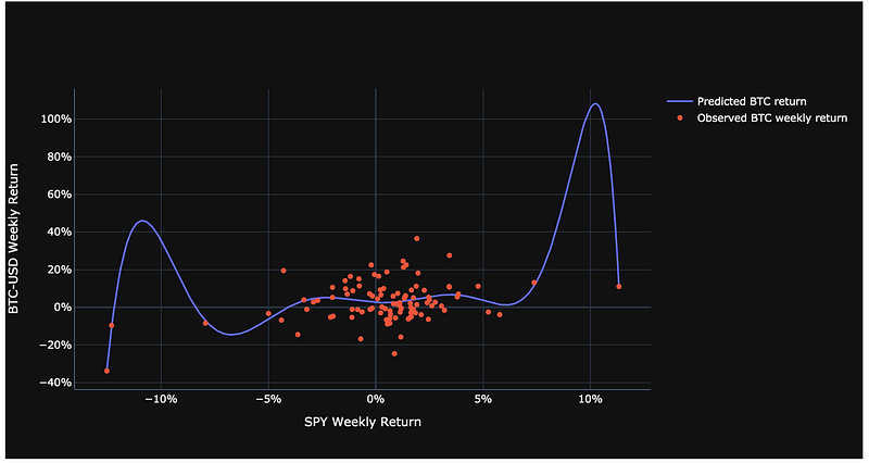

polyreg.score(X=df_X.values[:,0].reshape(-1,1), y=df_y.values[:,0])

This predictive model is massively overfitted, which makes this model nonsensical. When deploying machine learning algorithms, it is important to keep in mind that there are ways you can make your model fit the data better but that may result in nonsensical and poor predictions.

A regularization is a form of regression algorithm that helps guard against overfitting your model to noise in the training data. Examples of this are Ridge Regression and LASSO (least absolute shrinkage and selection operator) Regression. Essentially, they shrink the estimated coefficients towards 0 penalizing a more complicated model and this can give you a better chance for a more simple and robust model.

Ridge Regression is a popular type of regularized linear regression that includes an L2 penalty. An L2 penalty minimizes the size of all coefficients, although it prevents any coefficients from being removed from the model by allowing their value to become zero. This has the effect of shrinking the coefficients for those input variables that do not contribute much to the prediction task.

LASSO is a popular type of penalized regression where the penalty term involves summing the absolute values of the regression coefficients. The greater the number of included features, the larger the penalty. So, a feature must make a sufficient contribution to model fit to offset the penalty from including it.

Therefore, penalized regression ensures that a feature is included only if the sum of squared residuals declines by more than the penalty term increases. All types of penalized regression involve a trade-off of this type. Also, since LASSO eliminates the least important features from the model, it automatically performs feature selection.

Regularization methods can also be applied to non-linear models. A long-term challenge of the asset management industry in applying mean-variance optimization has been the estimation of stable covariance matrixes and asset weights for large portfolios. Asset returns typically exhibit strong multicollinearity, estimating the covariance matrix highly sensitive to noise and outliers, so the resulting optimized asset weights are highly unstable. Regularization methods have been used to address this problem.

Example 3: Forward Annual Dividend Yield vs Payout Ratio

In the final example, we regress the Forward Annual Dividend Yield versus the Payout Ratio for a group of stocks known to pay dividends consistently over time. We will first plot and regress our data for each stock.

We then build a multivariate regression that will first fit a train data set and then be used against a test data set to make predictions. We will analyze each feature to see which feature has a stronger relationship with predicting the response variable Y.

We can use the Key Statistics endpoint from the AlphaWave Data Stock Analysis API to pull in the required stock information.

#stocks for dividend analysis
dividend_stock_tickers = ['MMM','KO','CL','DOV','EMR','GPC','JNJ','PG','SWK','HRL','BDX',
'ITW','LEG','PPG','TGT','GWW','ABBV','ABT','FRT','KMB','PEP',
'VFC','NUE','SPGI','ADM','ADP','ED','LOW','WBA','CLX','MCD',
'PNR','WMT','MDT','SHW','SYY','BEN','CINF','AFL','APD','XOM',
'AMCR','T','BF-B','CTAS','ECL','MKC','TROW','CAH','CVX','ATO',
'GD','WST','AOS','LIN','ROP','CAT','CB','PBCT','ALB','ESS',
'EXPD','O','IBM','NEE']

url = "https://stock-analysis.p.rapidapi.com/api/v1/resources/key-stats"

headers = {
    'x-rapidapi-host': "YOUR_X-RAPIDAPI-HOST_WILL_COPY_DIRECTLY_FROM_RAPIDAPI_PYTHON_CODE_SNIPPETS",
    'x-rapidapi-key': "YOUR_X-RAPIDAPI-KEY_WILL_COPY_DIRECTLY_FROM_RAPIDAPI_PYTHON_CODE_SNIPPETS"
    }

dividend_stock_frames = []

for ticker in dividend_stock_tickers:
    querystring = {"ticker":ticker}
    dividend_stock_key_stats_response = requests.request("GET", url, headers=headers, params=querystring)
    time.sleep(2)

try:
        # Create Key Statistics DataFrame
        dividend_stock_key_stats_df = pd.DataFrame.from_dict(dividend_stock_key_stats_response.json())
        dividend_stock_key_stats_df = dividend_stock_key_stats_df.transpose()
        dividend_stock_key_stats_df = dividend_stock_key_stats_df.rename(columns={'Value':ticker})
        dividend_stock_frames.append(dividend_stock_key_stats_df)
    except:
        continue

dividend_stock_df = pd.concat(dividend_stock_frames, axis=1, join="inner")
dividend_stock_df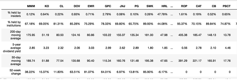

#convert the dataframe to include features we are interested in and prepare for analysis

dividend_stock_analysis_df = dividend_stock_df.transpose()
dividend_stock_analysis_df = dividend_stock_analysis_df.reset_index()
dividend_stock_analysis_df = dividend_stock_analysis_df.rename(columns={'index':'Symbol'})

dividend_stock_analysis_df = dividend_stock_analysis_df[['Symbol',
'Forward annual dividend yield ','Payout ratio ','Total debt/equity (mrq)','Operating margin (ttm)']]

dividend_stock_analysis_df = dividend_stock_analysis_df.replace(r'[%]+$', '', regex=True)
dividend_stock_analysis_df['Forward annual dividend yield '] = dividend_stock_analysis_df['Forward annual dividend yield '].astype(float)/100
dividend_stock_analysis_df['Operating margin (ttm)'] = dividend_stock_analysis_df['Operating margin (ttm)'].astype(float)/100
dividend_stock_analysis_df['Payout ratio '] = dividend_stock_analysis_df['Payout ratio '].astype(float)

dividend_stock_analysis_df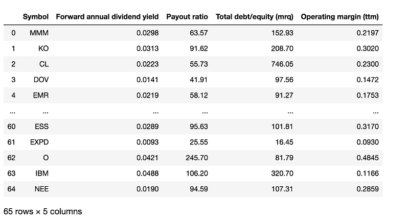

Instead of looking at the entire data as a whole, a lowess regression is a moving regression that looks at localized subsets of the data and does a weighted regression over those subsets. It then fuses those subsets. Although this is harder to represent mathematically, it may be warranted in certain situations.

In the two graphs below, you can see that the non-linear regression using a lowess regression fits the data better than a line created using an ordinary least squares regression.

#lowess regression

fig = px.scatter(
    dividend_stock_analysis_df, x='Payout ratio ', y='Forward annual dividend yield ',
    trendline='lowess', trendline_color_override='red'
)
fig.update_layout(template='plotly_dark', xaxis_title="Payout Ratio", yaxis_title="Forward Annual Dividend Yield",yaxis_tickformat = '.2%',xaxis_tickformat = '.2f')
fig.show()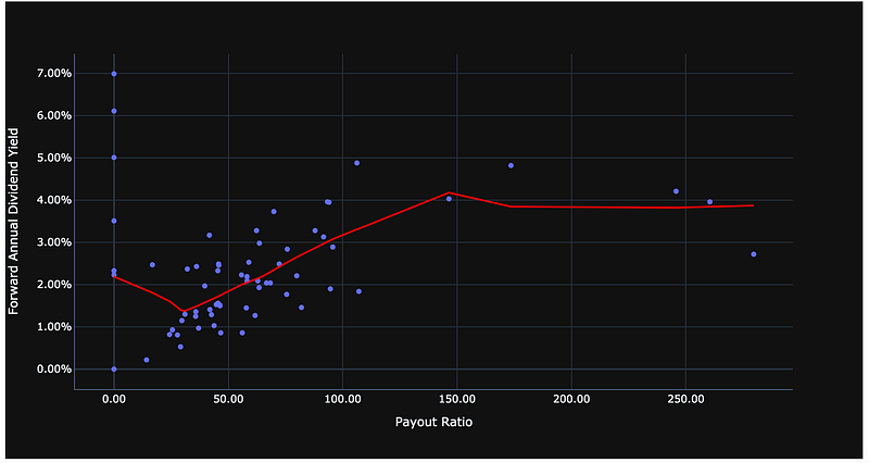

#ordinary least squares regression
fig = px.scatter(
    dividend_stock_analysis_df, x='Payout ratio ', y='Forward annual dividend yield ',
    trendline='ols', trendline_color_override='red'
)
fig.update_layout(template='plotly_dark', xaxis_title="Payout Ratio ", yaxis_title="Forward Annual Dividend Yield",yaxis_tickformat = '.2%',xaxis_tickformat = '.2f')
fig.show()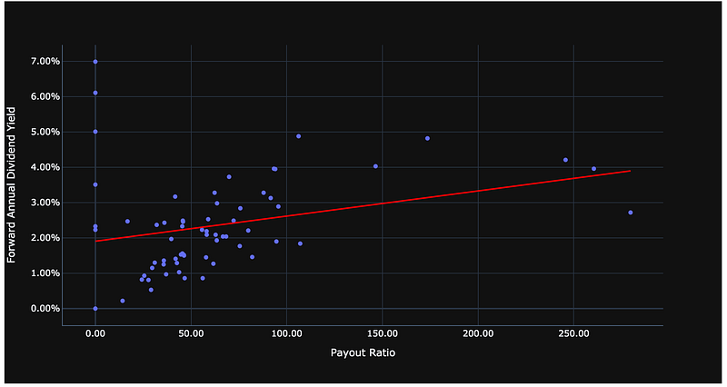

Fit the OLS model, and print the coefficients Slope and Intercept:

#Fit the OLS model using sklearn.linear_model.LinearRegression
X = dividend_stock_analysis_df['Payout ratio '].values.reshape(-1, 1)
y = dividend_stock_analysis_df['Forward annual dividend yield '].values
model = LinearRegression()
model.fit(X,y)

#Model Coefficients
print('Slope: {:.4f}'.format(model.coef_[0]))
print('Intercept: {:.4f}'.format(model.intercept_))

Use the model to predict the Forward Annual Dividend Yield of a stock with a hypothetical Payout Ratio of 150:

model.predict([[150]])

Residuals are the difference between observed data and the data predicted by our model. Note any patterns in the residuals. To make a good regression, the residuals should be randomly distributed, like random noise. If there is a predictable bias in the residuals (such as if all the points to the left are consistently below the predicted levels, thus all having negative residuals), that will translate to a biased model as seen in this example.

#Compute residuals as observed Forward Annual Dividend Yields minus
#the Forward Annual Dividend Yields predicted by the model
residuals = y - model.predict(X)

#Construct regression line from the model
x_vals_line = [dividend_stock_analysis_df['Payout ratio '].min(),dividend_stock_analysis_df['Payout ratio '].max()]
y_vals_line = model.predict(np.array(x_vals_line).astype(float).reshape(-1,1)).tolist()

#Plot
fig = go.Figure()
fig.add_trace(go.Scatter(x=dividend_stock_analysis_df['Payout ratio '].tolist(),y=dividend_stock_analysis_df['Forward annual dividend yield '].tolist(),mode='markers',name='Forward annual dividend yield'))
fig.add_trace(go.Scatter(x=x_vals_line, y=y_vals_line, name='Regression line', mode='lines'))
fig.add_trace(go.Bar(x=dividend_stock_analysis_df['Payout ratio '].tolist(),y=residuals.tolist(),width=3, name='Residuals'))
fig.update_layout(template='plotly_dark', xaxis_title="Payout Ratio", yaxis_title="Forward Annual Dividend Yield", yaxis_tickformat = '',xaxis_tickformat = '')
fig.show()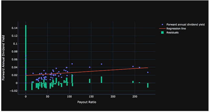

In addition to forwarding the Annual Dividend Yield and Payout Ratio, we also retrieved the stock’s Operating Margin and Debt to Common Equity Ratio to perform a multivariate regression.

We first separate the data into two partitions, training data and test data.

i_max_of_train_data = math.ceil(len(dividend_stock_analysis_df.dropna())/2)
df_train_data = dividend_stock_analysis_df.dropna().iloc[0:i_max_of_train_data]
df_train_data.count()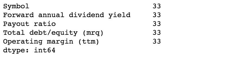

df_test_data = dividend_stock_analysis_df.dropna().iloc[i_max_of_train_data:]
df_test_data.dropna().count()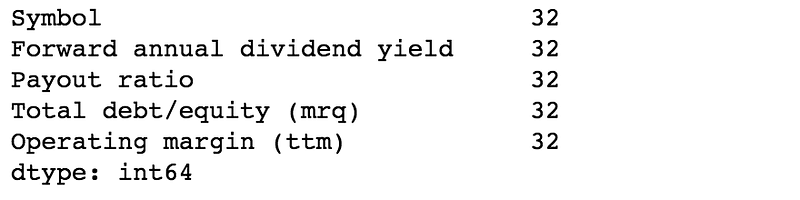

Now, we fit the multivariate regression model to the training data set.

df_train_data.head()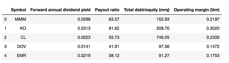

#Multivariate Regression on Z_Spread against duration, Amount Outstanding, and Debt to Common Equity Ratio
y = df_train_data['Forward annual dividend yield ']
x = df_train_data[['Payout ratio ','Total debt/equity (mrq)','Operating margin (ttm)']]

#Define multiple linear regression model (using sklearn library)
linear_regression = LinearRegression()

#Fit the multivariate linear regression model
linear_regression.fit(x,y)

Estimated coefficients of our model:

linear_regression.coef_

R squared of the fit on training data:

linear_regression.score(x,y)

We can now use our model to predict the Forward Annual Dividend Yield for a hypothetical stock with the below-chosen inputs for Payout Ratio, Debt to Common Equity Ratio, and Operating Margin.

linear_regression.predict([[150,500,0.25]])

Note that above we fitted the model on the training data set. Next, we apply the model to the separate test data set’s three features (Payout Ratio, Debt to Common Equity Ratio, and Operating Margin), to get a Predicted Forward Annual Dividend Yield for each stock in the test data set.

df_sub_test = df_test_data[['Payout ratio ','Total debt/equity (mrq)',\
                            'Operating margin (ttm)','Forward annual dividend yield ']].astype(float).copy()

#put test data into correct configuration to feed into model
l_features=['Payout ratio ','Total debt/equity (mrq)','Operating margin (ttm)']
num_features =3
l_lists = list()
for i in range(len(df_sub_test)):
    l_i = list()
    for i_feat in range(num_features):
        l_i.append(df_sub_test.iloc[i].loc[l_features[i_feat]])
    l_lists.append(l_i)

#predict values on test data set
predicted_vals = linear_regression.predict(l_lists)
df_sub_test = df_sub_test.assign(predicted_div_yield=predicted_vals)

df_sub_test.tail()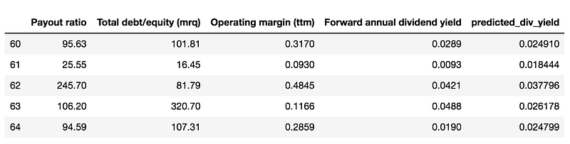

With a Predicted Forward Annual Dividend Yield for each stock in the test data set, we can plot the Predicted Forward Annual Dividend Yield and Observed Forward Annual Dividend Yield versus the Payout Ratio.

fig = go.Figure()

#dividend_plot
df = df_sub_test.sort_values('Payout ratio ')
fig.add_trace(go.Scatter(x=df['Payout ratio '],y=df['Forward annual dividend yield '],mode='markers',name='Observed Div Yield'))
fig.add_trace(go.Scatter(x=df['Payout ratio '],y=df['predicted_div_yield'],mode='markers',name='Predicted Div Yield'))
fig.update_layout(template='plotly_dark', xaxis_title="Payout Ratio", yaxis_title="Forward Annual Dividend Yield", yaxis_tickformat = '',xaxis_tickformat = '')
fig.show()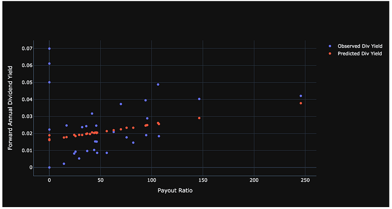

Since this is a multivariate regression, we can view the relationship for each variable to the Forward Annual Dividend Yield using the below code.

#Reshape data to produce a faceted plot
df_melted = df_sub_test.melt(id_vars=['Forward annual dividend yield ','predicted_div_yield'])

# Show faceted figure, with a plot for each of our features
fig = px.scatter(data_frame=df_melted,x='value',y=['Forward annual dividend yield ','predicted_div_yield'], facet_col='variable', template='plotly_dark')
fig.update_xaxes(matches=None)
fig.show()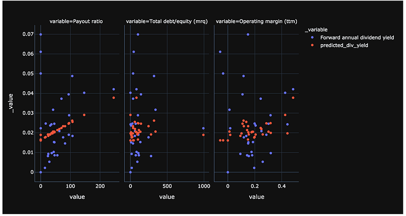

It appears that the Payout Ratio has a more significant relationship to the Forward Annual Dividend Yield than do the Debt to Common Equity Ratio and Operating Margin.

Conclusion

A regression model takes matched data (X’s, Y) and uses it to estimate parameters that characterize the relationship between Y and X’s. The estimated parameters can then be used to predict Y on a new, different set of Xs. The difference between the predicted and actual Y is used to evaluate how well the regression model predicts out-of-sample (i.e., using new data).

We looked at a linear regression of IBM returns versus SPY returns showing how to do this using SciPy, Scikit-learn, and NumPy libraries. Then, we analyzed the relationship between Bitcoin and SPY and talked through some of the pitfalls and reasons why regression may not work in all cases. In our third example, we built a multivariate regression to predict a stock’s Forward Annual Dividend Yield using its Payout Ratio, Debt to Common Equity Ratio, and Operating Margin.

As the first model typically introduced to those learning ML, regression is a technique to quantify what is observed in the world using a simplified model. The concepts introduced with regression can be drawn on when working with other ML techniques.

Additional Resources

Python Libraries

SciPy Linear Regression: https://docs.scipy.org/doc/scipy/reference/generated/scipy.stats.linregress.html

Scikit-learn Linear Regression: https://scikit-learn.org/stable/modules/generated/sklearn.linear_model.LinearRegression.html

Scikit-learn ML Packages: https://scikit-learn.org/stable/supervised_learning.html

Ridge Regression in Scikit-learn (Regularization): https://scikit-learn.org/stable/modules/generated/sklearn.linear_model.Ridge.html

LASSO Regression in Scikit-learn (Regularization): https://scikit-learn.org/stable/modules/generated/sklearn.linear_model.Lasso.html

ML Regression in Plotly: https://plotly.com/python/ml-regression/

This presentation is for informational purposes only and does not constitute an offer to sell, a solicitation to buy, or a recommendation for any security; nor does it constitute an offer to provide investment advisory or other services by AlphaWave Data, Inc. (“AlphaWave Data”). Nothing contained herein constitutes investment advice or offers any opinion concerning the suitability of any security, and any views expressed herein should not be taken as advice to buy, sell, or hold any security or as an endorsement of any security or company. In preparing the information contained herein, AlphaWave Data, Inc. has not taken into account the investment needs, objectives, and financial circumstances of any particular investor. Any views expressed and data illustrated herein were prepared based upon information, believed to be reliable, available to AlphaWave Data, Inc. at the time of publication. AlphaWave Data makes no guarantees as to its accuracy or completeness. All information is subject to change and may quickly become unreliable for various reasons, including changes in market conditions or economic circumstances.