
Introduction to Llama2 : Part-1 Architectural Analysis
Llama is a decoder-only language model, which takes the input sentence as ordered tokens and predicts the next token. In this article, we will be going through different components of the LLama architecture.

Figure 1 depicts the autoregressive nature of the Llama model. From the execution, we can understand that, the initial prefill sentence i.e. “The sun rises” is the first input to the model, and the model predicts the first output “in” as the next word. Further, the predicted word is used as input and the process continues until we encounter end-of-sentence(EOS) as output.
Inputs and Outputs to the model
As we know Machine Learning communicates in numbers, we can’t use the words directly as input. In this section, we will understand the inputs and outputs of Llama in detail.
Inputs
The model takes three inputs:
- Tokens
- Attention mask
- Positional Embedding
Tokens:
The input sentence is converted as a sequence of tokens using a tokenizer which internally uses a lookup table kind of mechanism.
Attention mask:
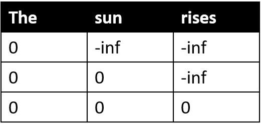
An attention mask is used to point out the importance of a particular word in the sentence with other words. From Figure.2 we can observe that the words ‘the’, ‘sun’, and ‘rises’ give attention to themselves and their predecessors only. This mask helps the model in doing generic calculations, instead of conditioning.
Positional Embedding
Positional embedding is used to give the model an idea about the positions of the words in the sentence, which helps to decide the importance of a word with other words based on the distance between them. Llama uses a new kind of positional embedding mechanism called Rotary Position Embedding(RoPE), which works in the angular domain instead of direct position weightage.
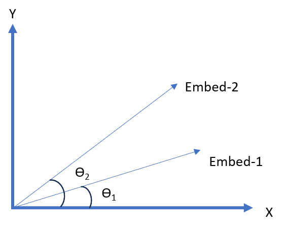
RoPE is used to transform or rotate the hidden-state embedding at a certain angle, and the angle is proportional to the position of the word in the sentence. The correlation between any two-embedding vectors is always proportional to COS(Ѳ2-Ѳ1), where Ѳ1 and Ѳ2 represents the angular rotation for a particular word embedding based on its position in the sentence. From the explanation, it is clear that the lesser the difference between angles Ѳ1 and Ѳ2 more the correlation, basically closer the words in the sentence more they are correlated.
Outputs:
The model outputs a token, which is then detokenized to a word using a de-tokenizer. If the new word is not EOS, it is again fed back to the model as new input.
Model Architecture
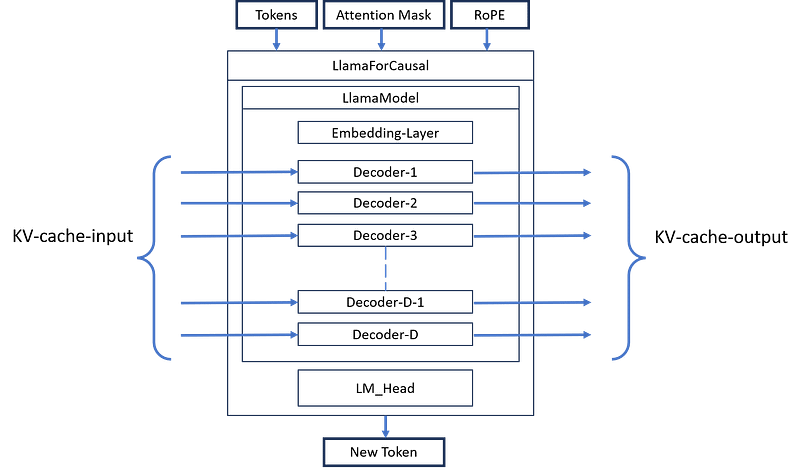
Figure 4 depicts the model architecture of Llama-2. The model contains an embedding layer followed by D number of decoder blocks and in the end, it has LM_Head which finally predicts the next token. We will be discussing each component in detail.
Embedding Layer
The embedding layer is a kind of lookup table that represents each token in a meaningful embedding vector. For example- In the Llama-2–7B model each word-token is represented in a 4096-dimensional embedding vector it is also called hidden_state size.
Decoder Block
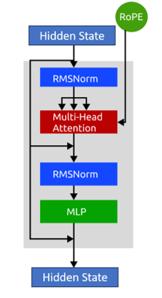
Decoder is the core block of the Llama model, it consists of RMSNorm, Multi-Head attention, and MLP layers. The output of one decoder block propagates to the next decoder block, like in Llama-2–7B model consists of 32 decoder blocks.
LM_Head
LM_Head is the last layer of Llama model, it is a linear layer that finally decodes the hidden states into tokens. The output dimension of LM_Head is always the same as the tokenizer dictionary size. This layer predicts the probabilities of tokens to be the next token.
The secret show:- KV-caching
From Figure 1 we can observe that for an Autocomplete use-case in the first step, we pass the input sentence “The sun rises” and based on this it predicts the next word ‘in’. Later in subsequent steps we pass the previously predicted word and get the next predicted word as output. Isn’t it magical? Who is guiding the model about the previously occurred words, or the context?. Here KV-caching comes into play. KV-caching is nothing but remembering the contexts in terms of some intermediate outputs. As explained in the previous sections the Llama-2 model consists of several decoder blocks containing attention and norm layers. To understand more we will be refreshing our transformer knowledge.
Self-Attention using Transformers:
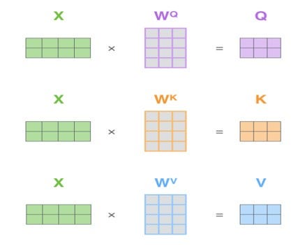
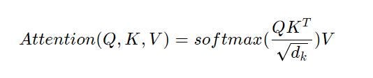
Figure 6 shows the Q, K, and V projections of the word embedding vector X, so if X has 3 word members for example in “The sun rises” it will have 3 rows in all Q, K, and Vs. We will take an example sentence and discuss about KV-caching.
Example
First Execution (Inside attention block):
Input sentence: “The sun rises” → X is 3 x k dimensional.
W(q), W(k), W(v) each one is k x z dimensional.
Q, K, and V each will be 3 x z dimensional.
The entity Q.(K^T) will be 3 x 3 dimensional, it decides the importance of each word with other words.
Finally, the entity Attention(Q, K, V) will be 3 x z dimensional.
After this, the K and V are stored as Past_K = K and Past_V = V to be used as context for the next word generation.
Subsequent Executions:
Input sentence: “in” → X is 1 x k dimensional.
Q-new, K-new, and V-new each will be 1x z dimensional.
Again the Q, K and V are updated as follows-
Q = Q-new, dim=1 x z
K = concat(Past_K, K-new) , dim = 4 x z
V = concat(Past_V, V-new), dim = 4 x z
The entity Q.(K^T) will be 1 x 4 dimensional, it decides the importance of the input word with other previously processed words.
Finally, the entity Attention(Q, K, V) will be 1 x z dimensional.
Here we avoid the recomputation of K and V during each execution, instead cache it as: Past_K = K and Past_V = V.
Big Question: Is it a generative model? How?
Since we can observe that for the same input we will be getting the same output every time, then the question arises “How, it is a generative model?”. Actually, to feed a generative behavior in the model we add an output wrapper called sampler, we will discuss this in the second part of the article.


