Introduction To Geospatial Analysis With Python

Learn how to use Python to create maps and visualize geographic information for data-driven discovery, visualize landscapes, and transform raw data into valuable knowledge

In this blog, we will cover the below topics

• What is Geospatial Analysis?
• What are the key components of Geospatial Analysis?
• What are the applications of Geospatial analysis?
• Why Python for Geospatial Analysis?
• Setting Up Your Geospatial Python Environment
• Loading and Visualizing Geospatial Data
• References and FAQs

What is Geospatial Analysis?

Geospatial analysis is a multidisciplinary approach that involves examining and interpreting data with a geographic or spatial component to uncover patterns, relationships, and insights about the Earth’s surface and its features. It combines geography, cartography, statistics, and technology to analyze and visualize various types of spatial data, such as maps, satellite imagery, GPS coordinates, and remote sensing data.

The primary goal of geospatial analysis is to gain a deeper understanding of the spatial distribution and interconnections between different phenomena. This approach enables researchers, analysts, and decision-makers to address complex questions related to urban planning, environmental monitoring, disaster management, resource allocation, transportation optimization, and much more.

What are the key components of Geospatial Analysis?

The geospatial analysis encompasses several key components.

Data Collection: Gathering spatial data from various sources, including satellites, surveys, sensors, and mobile devices. This data may include geographic features (e.g., rivers, roads, buildings), attributes (e.g., population density, land use), and temporal information.

Data Integration and Management: Organizing and storing spatial data in geographic information systems (GIS) or specialized databases, enabling efficient retrieval and manipulation.

Spatial Analysis: Applying statistical and computational methods to examine spatial relationships, patterns, and trends. This can involve proximity analysis, spatial interpolation, clustering, and spatial modeling.

Visualization: Creating maps, charts, and graphs to represent geospatial data visually. Visualization helps in communicating complex spatial information in a comprehensible manner.

Decision Support: Geospatial analysis aids in making informed decisions by providing insights into the spatial implications of various choices. For instance, it can help determine the best location for a new retail store based on demographic data and competitor locations.

Predictive Modeling: Using historical geospatial data to create models that forecast future trends or events, such as predicting disease outbreaks based on patterns of past occurrences.

What are the applications of Geospatial analysis?

Geospatial analysis finds diverse applications across various sectors, leveraging spatial data to gain valuable insights and inform decision-making. Here are the top five applications of geospatial analysis:

Urban Planning and Development: Geospatial analysis helps urban planners optimize land use, infrastructure development, and transportation systems. It aids in identifying suitable locations for new buildings, roads, and public services, as well as predicting population growth patterns to ensure sustainable urban development.

Natural Resource Management: This application involves monitoring and managing natural resources such as forests, water bodies, and agricultural lands. Geospatial analysis assists in assessing land cover changes, tracking deforestation, estimating water availability, and implementing conservation strategies.

Disaster Management and Emergency Response: Geospatial analysis plays a vital role in disaster preparedness and response. It helps track the movement of natural disasters (e.g., hurricanes, wildfires), assess damage, and allocate resources effectively during emergencies.

Environmental Monitoring and Conservation: Conservationists and environmental agencies use geospatial analysis to monitor biodiversity, track wildlife habitats, and analyze changes in ecosystems. It aids in identifying areas of concern and planning conservation efforts.

Public Health: Geospatial analysis is employed to understand the spread of diseases, track outbreaks, and assess healthcare accessibility. It assists in mapping disease patterns and predicting the potential impact of health crises.

Why Python for Geospatial Analysis?

Python has emerged as a dominant force in geospatial analysis, largely due to its extensive range of purpose-built libraries and user-friendly syntax. Python is particularly enticing for both newcomers and seasoned programmers alike, thanks to its intuitive syntax that fosters accessible and collaborative geospatial exploration.

• Open Source: Python is open-source and freely available, which lowers the entry barrier for individuals and organizations to start using it for geospatial analysis. This fosters a collaborative community that contributes to the development and improvement of geospatial tools.
• Interoperability: Python’s libraries allow for seamless integration with other data analysis and visualization tools. This makes it easy to combine geospatial analysis with statistical analysis, machine learning, and data visualization tasks.
• Rich Geospatial Libraries: Python boasts a robust ecosystem of geospatial libraries that provide various functionalities for data manipulation, analysis, and visualization. Notable libraries like GDAL, Shapely and GeoPandas
• Data Visualization: Python offers libraries like Matplotlib, Seaborn, Plotly, and Folium for creating visualizations that enhance the interpretation of geospatial data. These libraries enable you to generate maps, charts, and graphs to communicate your findings effectively.

Let’s try a few examples with Python code in the next section.

Setting up Python environment

Set up your development environment

Let us create a virtual environment, we will use the same environment for all the use cases that follow in the subsequent sections. Here are the steps to create a virtual development environment.

# STEP 1: Open the terminal and install the library virtualenv
pip install virtualenv

# STEP 2: Create a new virtual environment
virtualenv geospatial

# STEP 3: Activate the new virtual environment
geospatial\scripts\activate

Importing the libraries

We will need two Python libraries GeoPandas for spatial analysis and Matplotlib for visualization.

GeoPandas: It is an open-source Python library that provides an easy and efficient way to work with geospatial data. It builds upon the capabilities of two popular libraries, pandas (for data manipulation) and shapely (for geometry operations), to enable users to manage, analyze, and visualize geographic data seamlessly within a familiar data analysis environment.

Matplotlib: It is a widely used open-source Python library that provides comprehensive tools for creating static, interactive, and animated visualizations in a variety of formats.

# pip install geopandas
import geopandas as gpd
 
# pip install matplotlib
import matplotlib.pyplot as plt

Visualizing Geospatial data

Let’s start with the basic world map. We will use the built-in dataset from GeoPandas. We can change the camp configuration to try various other color ranges but for now, let's use “OrRd”.

world = gpd.read_file(gpd.datasets.get_path('naturalearth_lowres'))
fig, ax = plt.subplots(figsize=(10, 8))
world.plot(ax=ax, cmap = 'OrRd')
plt.show()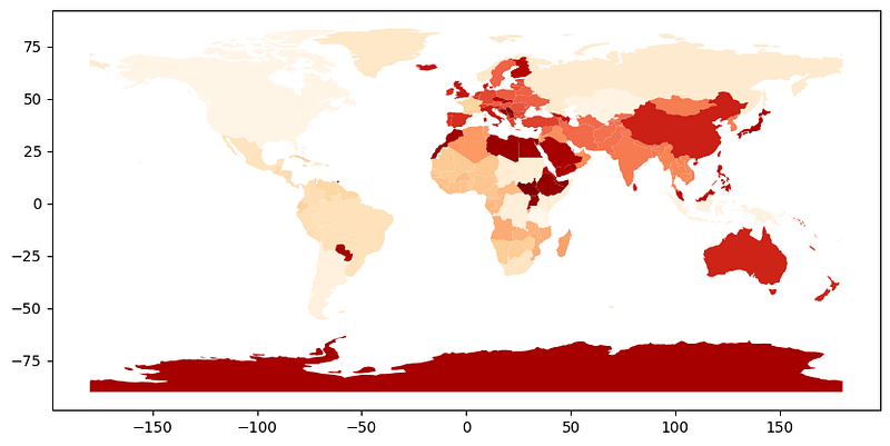

We can also pick a specific country and carry out the analysis. Let’s try this with Belgium. We will use the shapefile for Belgium.

Belgium = gpd.read_file("BEL_adm/BEL_adm1.shp")
Belgium.head()

OUTPUT:
 ID_0 ISO NAME_0 ID_1 NAME_1 TYPE_1 ENGTYPE_1 NL_NAME_1 VARNAME_1 geometry
0 23 BEL Belgium 1 Bruxelles Gewest Region NaN Brussel POLYGON ((4.40986 50.90990, 4.41251 50.90924, ...
1 23 BEL Belgium 2 Vlaanderen Gewest Region NaN Flandres MULTIPOLYGON (((5.78851 50.77223, 5.79070 50.7...
2 23 BEL Belgium 3 Wallonie Région Region NaN NaN MULTIPOLYGON (((3.03365 50.77507, 3.03668 50.7...

We find that there are 3 states or territories namely Bruxelles, Vlaanderen, and Wallonie. Let's visualize them on the map

Belgium["coords"] = Belgium["geometry"].apply(lambda x: x.representative_point().coords[:])
Belgium["coords"] = [coords[0] for coords in Belgium["coords"]]

fig, ax = plt.subplots(figsize = (6,6))
Belgium.plot(ax=ax, cmap='viridis')

for idx, row in Belgium.iterrows():
    plt.annotate(text=row["NAME_1"], xy=row["coords"], 
                horizontalalignment="center", color = "purple")

plt.show()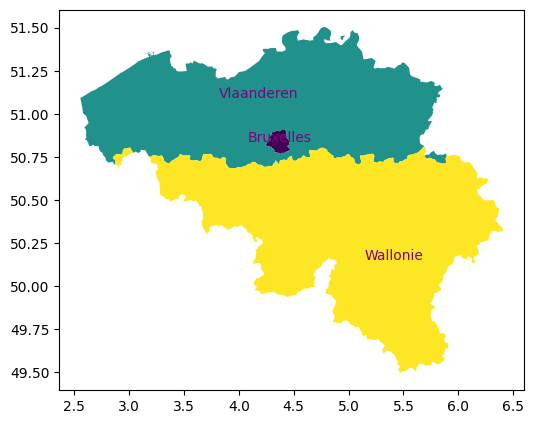

Let's drill deeper into Wallonie and look at the territories in detail.

state = Belgium[Belgium['NAME_1'] == 'Wallonie']
state.plot(cmap='viridis', figsize=(5, 5))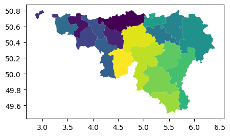

We can now analysis for various Belgium territory-specific use cases for eg: showcasing population density, crime rates, mineral reservoirs, per capita income, seismic activity, etc on the map.

As we near the end of the blog, let’s use all that we have learned and apply it to a use case by visualizing the seismic activity on the world map. We could do that with a few lines as below.

1. We will fetch the data from USGS URL and then load it to earthquake_data. This has 22 columns covering various parameters including latitude, longitude, place, etc. Once the data is loaded, it appears like a typical data frame but it isn’t. This is in the GeoDataFrame

# Load the data
url = "https://earthquake.usgs.gov/earthquakes/feed/v1.0/summary/all_month.csv"
earthquake_data = pd.read_csv(url)


OUTPUT:
type(earthquake_data)
geopandas.geodataframe.GeoDataFrame

time latitude longitude depth mag magType nst gap dmin rms ... updated place type horizontalError depthError magError magNst status locationSource magSource
0 2023-08-16T12:51:42.418Z 60.466800 -150.859600 53.70 3.90 ml NaN NaN NaN 0.27 ... 2023-08-16T12:55:24.848Z Kenai Peninsula, Alaska earthquake NaN 1.60 NaN NaN automatic ak ak
1 2023-08-16T12:32:13.886Z 62.522900 -149.465600 37.70 1.30 ml NaN NaN NaN 1.17 ... 2023-08-16T12:34:21.298Z 33 km ENE of Chase, Alaska earthquake NaN 3.30 NaN NaN automatic ak ak
2 2023-08-16T11:27:09.745Z 62.379000 -148.199700 36.80 1.40 ml NaN NaN NaN 0.84 ... 2023-08-16T11:29:30.025Z 66 km NNE of Chickaloon, Alaska earthquake NaN 1.10 NaN NaN automatic ak ak
3 2023-08-16T11:25:28.720Z 33.311667 -116.354167 9.55 1.19 ml 47.0 40.0 0.06829 0.18 ... 2023-08-16T12:42:40.816Z 6 km NNE of Borrego Springs, CA earthquake 0.25 0.55 0.138 26.0 reviewed ci ci
4 2023-08-16T11:09:15.140Z 33.343667 -116.270000 6.19 0.68 ml 30.0 141.0 0.14440 0.25 ... 2023-08-16T11:12:46.762Z 14 km NE of Borrego Springs, CA earthquake 0.45 1.69 0.192 11.0 automatic ci ci

2. We plan to showcase the earthquake locations on the world point which means we will need the latitude and longitude information and this should be in the form of point geometries (like an array). This will be added as an additional column in the GeoDataFrame.

geometry = gpd.points_from_xy(earthquake_data.longitude, 
                              earthquake_data.latitude)

OUTPUT:
<GeometryArray>
[ <POINT (-150.86 60.467)>, <POINT (-149.466 62.523)>,
   <POINT (-148.2 62.379)>, <POINT (-116.354 33.312)>,
  <POINT (-116.27 33.344)>,  <POINT (-116.15 33.769)>,
 <POINT (-118.292 35.481)>, <POINT (-155.407 19.207)>,
 <POINT (-83.742 -41.193)>, <POINT (-121.193 35.764)>,
 ...
  <POINT (-155.157 58.24)>, <POINT (-149.957 61.665)>,
 <POINT (-121.306 36.785)>, <POINT (-161.116 54.762)>,
 <POINT (179.857 -25.387)>,    <POINT (-98.14 35.65)>,
 <POINT (-165.934 54.171)>, <POINT (-160.956 54.619)>,
  <POINT (-155.155 58.25)>, <POINT (-149.043 60.696)>]
Length: 10451, dtype: geometry


earthquakes = gpd.GeoDataFrame(earthquake_data, geometry=geometry)

3. Visualize the earthquake locations on the world map

fig, ax = plt.subplots(figsize=(10, 8))
world.plot(ax=ax,  color='lightgrey')
# plt.show()
earthquakes.plot(ax=ax, markersize=earthquakes['mag']*2, color='red', 
                                                        alpha=0.5)
plt.title("Earthquake Activity Map")
plt.xlabel("Longitude")
plt.ylabel("Latitude")
plt.show()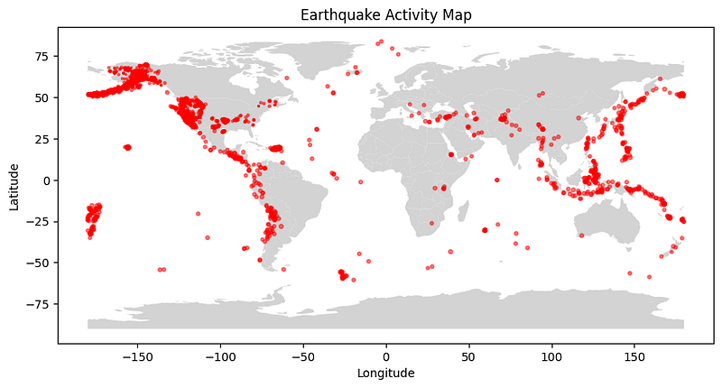

Conclusion

To summarize, delving into geospatial analysis with Python opens up a world of possibilities. Python’s special tools make it easier to understand and work with geographic data. From studying maps to understanding how cities grow, Python helps us uncover hidden patterns in our world. We can create maps that tell stories and predict future trends. The combination of Python’s easy-to-learn language and powerful libraries like GeoPandas allows us to explore and solve real-world problems. So, whether you’re a budding explorer or a curious mind, Python is your compass to navigate the exciting world of geospatial analysis.

I hope you liked the article and found it helpful.

You can connect with me — on Linkedin and Github

My other Geospatial Analysis blogs

Visualizing Geospatial Information using GeoPandas in Python Interactive Geospatial Maps using Folium in Python

References

GeoPandas

Matplotlib

FAQ

Q1: What are the other tools and software for Geospatial analysis? A1: Programming language like R is popular that is similar to Python. Also, tools like ArGis, QGis, and MATLAB are other options to consider

Q2: What is the learning curve for Geospatial analysis? A2: The learning curve for geospatial analysis can vary widely depending on factors such as your prior background, the complexity of the tasks you want to accomplish, the tools you choose to use, and the depth of analysis you aim to achieve. Starting with simpler tasks and gradually building your skills as you gain confidence is a recommended approach.

Q3: What are shapefiles? A3: Shapefiles are a common file format used in geospatial analysis and Geographic Information Systems (GIS) to store and manage geospatial data. They were developed by Esri (Environmental Systems Research Institute) and have become a de facto standard for representing and exchanging geographic information.

In Plain English

Thank you for being a part of our community! Before you go:

• Be sure to clap and follow the writer! 👏
• You can find even more content at PlainEnglish.io 🚀
• Sign up for our free weekly newsletter. 🗞️
• Follow us on Twitter, LinkedIn, YouTube, and Discord.