Hands-on Tutorial

Introduction to Fuzzy c-means for Clustering Algorithm

Basic introduction and implementation of Fuzzy c-means clustering algorithm using Python

There are a lot of clustering algorithms out there for the numerical data type. The k-means is one of the basic clustering algorithms that is commonly used by the researcher or analyst. But have you ever heard about the Fuzzy c-means before for clustering? If you haven’t, this article is for you.

In this short article, you will explore the Fuzzy c-means, starting from the basic structure of fuzzy, manual calculation and formula of Fuzzy c-means, and the implementation of Fuzzy c-means in Python using dummy data.

Okay, without further ado, let’s jump in!

Hard partition vs. fuzzy partition

Before talking about the basic theory of Fuzzy c-means, firstly better we talk about how the data points are theoretically allocated into clusters. Basically, there are two approaches, hard partition and fuzzy partition.

Hard partition — where the data points are strictly allocated as a member of one cluster and are not a member of another cluster, assuming that the number of clusters is known. The k-means is one of the algorithms that use a hard partition.

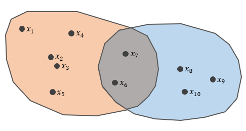
For instance, there are X = {x1, x2, …, x10}. They will be assigned into two clusters, let’s say cluster 1 and cluster 2. However, x6 and x7 are unfortunately in a grey area of two clusters.

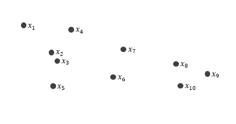
Let’s say U is the partition matrix for X. Thus, the elements of matrix U will be as follows. The columns represent the data points while the rows are the clusters.

Clusters using hard partition (Image by Author)

Remember that in a hard partition, there are only binary values [0, 1] so every data point must be assigned to one cluster. In this case, x6 is in cluster 1 while x7 is in cluster 2.

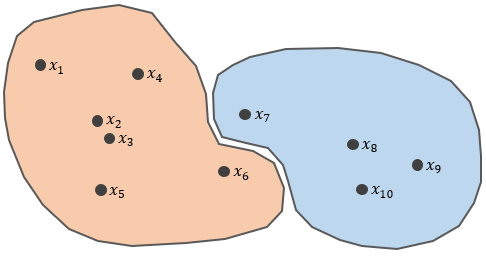
Visualization of clusters using hard partition (Image by Author)

Fuzzy partition — where every data point is given a probability of closeness [0, 1] for existing clusters, assuming that the number of clusters is known. One of the algorithms that use fuzzy partition is Fuzzy c-means that we will talk about it in depth.

For instance, using the previous case, we have X = {x1, x2, …, x10}.

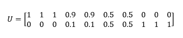
Clusters using fuzzy partition (Image by Author)

Look at x6 and x7 where they are in a grey area of two clusters. In fuzzy partition, they have a probability of 0.5 to be assigned in cluster 1 and 2. It will be fair for both of them.

Visualization of clusters using fuzzy partition (Image by Author)

The basic theory of Fuzzy c-means

Fuzzy c-means (FCM) was first introduced by Jim Bezdek in 1981. This method is an improvement of k-means by combining the fuzzy principle. Unlike the k-means, the data points that are clustered using FCM will become a member of each existing cluster. The dominant cluster for each data point is determined by the probability of its closeness which is in the range of 0 to 1.

In clustering, the k-means in allocating the data back into each cluster are based on the distance between the data and centroids in each existing cluster. The data is strictly reallocated to the cluster which has the closest centroids to the data points. Meanwhile, the FCM allocates the data points into each cluster by utilizing fuzzy theory. This theory generalizes the allocation method which is a hard partition used in k-means. In the FCM, membership functions are used, μ(x) which refers to how likely the data points can be the member of a certain cluster.

Optimal local solution versus optimal global solution (Image by Author)

Furthermore, theoretically, it is quite possible to fail to converge in the k-means and fuzzy c-means. In FCM, the possibility of this problem occurring is rare because each data point has a membership function to become a member of the cluster.

To understand the mathematical calculation of FCM, look at the following document.

Hands-on tutorial with Python

Firstly, some packages must be installed before going any further. This package list and its specifications are as follows. Important to note that there are other alternatives for fcmeans package, you can try them by yourself.

pandas — perform data frame manipulation
numpy — perform matrices operation (linear algebra)
sklearn — create dummy data for simulation using make_blobs and to rescale the data (numerical data type) using StandardScaler
fcmeans — perform the Fuzzy c-means clustering algorithm
plotly — create an interactive data visualization (in the 3D plot)

# Import packages
import pandas as pd
import numpy as np
from sklearn.datasets import make_blobs
from fcmeans import FCM
import plotly.graph_objects as go
from sklearn.preprocessing import StandardScaler

Next, using make_blobs we create a dummy data set that has three clusters. Further, it has 2,000 rows and 3 features or columns. To create overlapped data points, we can modify cluster_std (the greater value of cluster_std, the more overlapping data is generated).

# Generate dummy data
features, clusters = make_blobs(
    n_samples = 2000,
    n_features = 3,
    centers = 3,
    cluster_std = 0.8,
    shuffle = True,
    random_state = 0
)
# Concate these arrays
array = np.column_stack([features, clusters])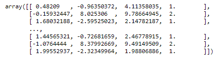

An array of dummy data (Image by Author)

Furthermore, we convert the array of previous dummy data into a data frame so we can easily manipulate and visualize it using pandas and plotly.

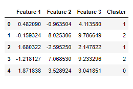
# Data frame
df = pd.DataFrame(
    data = array,
    columns = [
        'Feature 1',
        'Feature 2',
        'Feature 3',
        'Cluster'
    ]
)
# Change data type
df = df.astype(
    {
        'Cluster': object
    }
)
# Dimension of data
print('Dimension of data: {rows} rows and {columns} columns'.format(
        rows = len(df),
        columns = len(df.columns)
    )
)

The sample of dummy data (Image by Author)

The clusters are visually spread out (not overlapping). Each cluster can be easily distinguished from the others. It makes the Fuzzy c-means algorithm works easily in determining and assigning the clusters.

# Duplicate data
df_viz = df.copy()
# Set data size
df_viz['Size'] = df_viz.apply(
    lambda x: abs(x['Feature 1'] * x['Feature 2'] * x['Feature 3']),
    axis = 1
)
# Set the color
df_viz['Color'] = df_viz['Cluster'].map(
    {
        0: '#355C7D',
        1: '#F67280',
        2: '#F8B195'
    }
)
# Create object of figure
fig = go.Figure()
# Create a 3d scatter plot
fig.add_trace(
        go.Scatter3d(
            x = df_viz['Feature 1'],
            y = df_viz['Feature 2'],
            z = df_viz['Feature 3'],
            mode = 'markers',
            marker = {
                'size': 5,
                'color': df_viz['Color']
            },
            hovertemplate = 
            '<b>Feature 1:</b> %{x:}<br>' +
            '<b>Feature 2:</b> %{y:}<br>' +
            '<b>Feature 3:</b> %{z:}' +
            '<extra></extra>'
        )
    )
# Config for background etc
fig.update_layout(
    scene = {
        'xaxis': {
            'title': 'Feature 1'
        },
        'yaxis': {
            'title': 'Feature 2'
        },
        'zaxis': {
            'title': 'Feature 3'
        }
    },
    margin = {
        'l': 0,
        'r': 0,
        'b': 0,
        't': 0
    }
)

While the value range of data points in all columns varies, we should perform data standardization or data rescaling. It will anticipate the error in calculating the distance matrix. For instance, a column with a larger value range will dominate the other columns, thus it’s not fair in determining the clusters.

# Select columns for clustering
cols = ['Feature 1', 'Feature 2', 'Feature 3']
# Filter the columns and convert into matrix
df_not_scaled = df[cols].to_numpy()
# Min-max scaler
scaler = StandardScaler()
# Transform the data
scaled = scaler.fit_transform(df_not_scaled)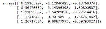

The sample of dummy data after rescaling (Image by Author)

In this case, we have already known the number of clusters that should be generated. However, what if we don’t know it yet? Okay, we can consider using the following methods. These can give us the insight to specify the appropriate number of clusters.

Elbow
Average silhouette
Gap statistic

The fcm is a cluster object we created for assigning the parameters for clustering analysis, such as the number of clusters and random state for randomization).

# Fit the cluster
fcm = FCM(n_clusters = 3, random_state = 0)
fcm.fit(scaled)

After the fitting has been completed, we can print the cluster centroids for each cluster. Because we have 3 features and 3 clusters, we get an array of n x m (n represents the number of clusters while m is the number of columns).

# Cluster centorids
fcm.centers

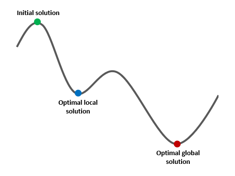
Cluster centroids generated using Fuzzy c-means (Image by Author)

In this data set, the Fuzzy c-means algorithm stops when the error reaches 0.00001. When this algorithm is too sensitive to local optimal, we can’t conclude that this is the best solution or the smallest error. However, the result is good for the benchmarks if we consider the next improvement.

# Check the error of the clusters generated
fcm.error

# Output
# 1e-05

Finally, we can assign the cluster labels to the dummy data to visualize them in a 3D plot. Further, to obtain the labels, we run the predict method in the cluster object of fcm.

# Predict the clusters
cluster_labels = fcm.predict(scaled)
# Add the cluster to the dataframe
df['Cluster FCM'] = cluster_labels

If we look carefully at the following 3D plot, we will find a data point that is clustered incorrectly. It should be in a blue cluster but is in a cream cluster. Visually, its location is far away from the cream cluster centroids.

# Duplicate data
df_viz = df.copy()
# Set the color
df_viz['Color FCM'] = df_viz['Cluster FCM'].map(
    {
        0: '#355C7D',
        1: '#F67280',
        2: '#F8B195'
    }
)
# Create object of figure
fig = go.Figure()
# Create a 3d scatter plot
fig.add_trace(
        go.Scatter3d(
            x = df_viz['Feature 1'],
            y = df_viz['Feature 2'],
            z = df_viz['Feature 3'],
            mode = 'markers',
            marker = {
                'size': 5,
                'color': df_viz['Color FCM']
            },
            hovertemplate = 
            '<b>Feature 1:</b> %{x:}<br>' +
            '<b>Feature 2:</b> %{y:}<br>' +
            '<b>Feature 3:</b> %{z:}' +
            '<extra></extra>'
        )
    )
# Config for background etc
fig.update_layout(
    scene = {
        'xaxis': {
            'title': 'Feature 1'
        },
        'yaxis': {
            'title': 'Feature 2'
        },
        'zaxis': {
            'title': 'Feature 3'
        }
    },
    margin = {
        'l': 0,
        'r': 0,
        'b': 0,
        't': 0
    }
)

Conclusion

One of the advantages of FCM is the implementation of fuzzy partition so the data points can be overlapped on more than a single cluster. It impacts the membership of data points among the cluster — in other words, we can evaluate the sensitivity of data points membership from one cluster to another cluster. Nevertheless, according to the mathematical computation, the iteration is depending on the smallest tolerance error — if we set the error quite small then the running time will be longer.

References

Agustin T, Djuraidah A. 2010. Clustering backward region in Indonesia using fuzzy c-means cluster. Forum Statistika dan Komputasi. 15(1): 22–27.

Jang JSR, Sun CT, Mizutani E. 1997. Neuro-Fuzzy and Soft Computing: A Computational Approach to Learning and Machine Intelligence. New Jersey (USA): Prentice-Hall, Upper Saddle River.

Kirschfink H, Lieven K. 1999. Basic Tools for Fuzzy Modeling. https://citeseerx.ist.psu.edu/.

Sanusi W, Zaky A, Afni BN. 2019. Analisis fuzzy c-means dan penerapannya dalam pengelompokan kabupaten/kota di provinsi Sulawesi Selatan berdasarkan faktor-faktor penyebab gizi buruk. Journal of Mathematics, Computations, and Statistics. 2(1).