
Inside the Convolution: Building a Convolution Layer Using Numpy Arrays
See how different settings affect the output of the convolution layer

In my previous article, I explained what convolutions are and why they are so essential in computer vision. However, I didn’t get to work with some examples to show exactly how it happened. In the present post, I will explain how filters (kernels) go along the image data, and how the output is affected by different settings of the convolution layers such as kernel size or stride length.
For this purpose, we will use the simplest possible example. The image data will contain only one channel, and the convolution layer we will build will contain only one filter. The aim is to understand the basics!
In this article we will only need two libraries:
import numpy as np
import matplotlib.pyplot as np
We will use an image of the vowel ‘a’ in a 12x12 matrix in greyscale. To make things even simpler, the initial values of our initial image matrix are only 0 and 1:
# Create a 12x12 matrix with all values initialized to 0
matrix_a = np.zeros((12, 12), dtype=int)

# Set non-zero values at specified positions
positions = [(2, 4), (2, 5), (2, 6), (3, 3), (3, 7), (4, 2), (4, 7),
             (5, 2), (5, 7), (6, 2), (6, 7), (7, 3), (7, 6), (7, 7),
             (8, 8), (8, 9), (7, 10), (8, 4), (8, 5)]

for position in positions:
    matrix_a[position] = 1

# Print the resulting matrix
print(matrix_a)
The next step is to create our first filter with size 3x3, and a new variable to store the results of the convolution. The first filter will contain all values equal to 1 to simplify the calculations. The variable result is a 2D numpy array with the same size as matrix_a, but full of zeros.
# Convolution filter
filter_a = np.array([
    [1, 1, 1],
    [1, 1, 1],
    [1, 1, 1]
])

result = np.zeros_like(matrix_a)
Now we will create a convolution with the filter from the previous step using two for loops that will perform position-wise multiplications for every position in matrix_a. After the position-wise multiplication, the values in the filter are summed and this value is stored in the corresponding position of the result matrix. The code used here applies a stride length of 1, and as the filter advances to the next position no additional instructions are given.
# Perform convolution
for i in range(matrix_a.shape[0] - filter_a.shape[0] + 1):
    for j in range(matrix_a.shape[1] - filter_a.shape[1] + 1):
        result[i, j] = np.sum(matrix_a[i:i+filter_a.shape[0], j:j+filter_a.shape[1]] * filter_a)
We can print the result:
# Print the result
print(result)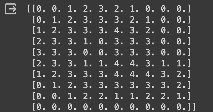
And we can also see what the old and new image looks like:
# Display the original 'a' and the result
plt.subplot(1, 2, 1)
plt.imshow(matrix_a, cmap='gray')
plt.title('Original "a"')

plt.subplot(1, 2, 2)
plt.imshow(result, cmap='gray')
plt.title('Convolution Result')

plt.show()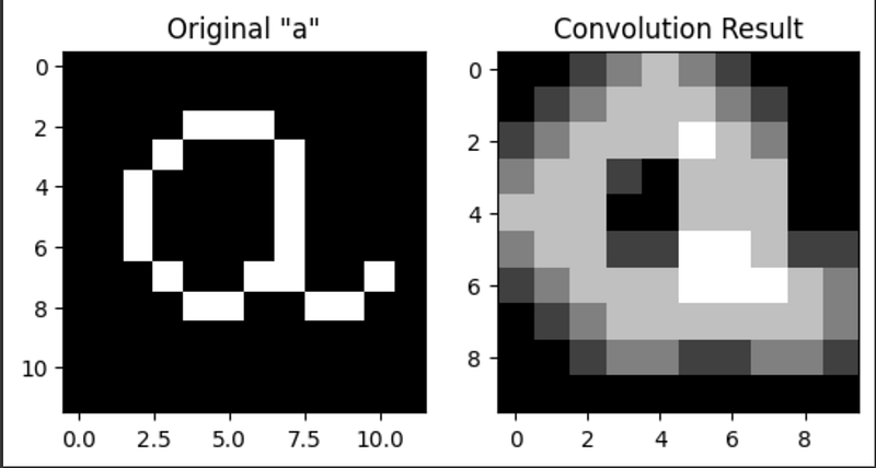
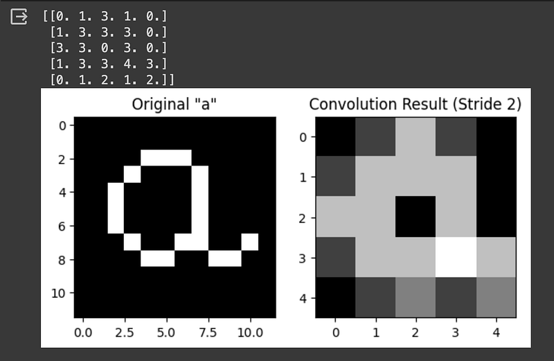
If we want to implement a different stride length, we need to add some code in the example given before and adjust the result's size. For a stride length of 2, we can use the following code:
# Perform convolution with stride of 2
result = np.zeros_like(matrix_a)

stride_length = 2
result = np.zeros((1 + (matrix_a.shape[0] - filter_a.shape[0]) // stride_length,
                   1 + (matrix_a.shape[1] - filter_a.shape[1]) // stride_length))

for i in range(0, matrix_a.shape[0] - filter_a.shape[0] + 1, stride_length):
    for j in range(0, matrix_a.shape[1] - filter_a.shape[1] + 1, stride_length):
        result[i // stride_length, j // stride_length] = np.sum(matrix_a[i:i+filter_a.shape[0], j:j+filter_a.shape[1]] * filter_a)

# Print the result
print(result)

# Display the original 'a' and the result
plt.subplot(1, 2, 1)
plt.imshow(matrix_a, cmap='gray')
plt.title('Original "a"')

plt.subplot(1, 2, 2)
plt.imshow(result, cmap='gray')
plt.title(f'Convolution Result (Stride {stride_length})')

plt.show()
Now the result is a 5x5 matrix according to the formula:
Output size = ((Input size — Kernel size) / Stride) + 1
We can go even further and try a stride length of 3:
# Perform convolution with stride of 3
result = np.zeros_like(matrix_a)

stride_length = 3
result = np.zeros((1 + (matrix_a.shape[0] - filter_a.shape[0]) // stride_length,
                   1 + (matrix_a.shape[1] - filter_a.shape[1]) // stride_length))

for i in range(0, matrix_a.shape[0] - filter_a.shape[0] + 1, stride_length):
    for j in range(0, matrix_a.shape[1] - filter_a.shape[1] + 1, stride_length):
        result[i // stride_length, j // stride_length] = np.sum(matrix_a[i:i+filter_a.shape[0], j:j+filter_a.shape[1]] * filter_a)

# Print the result
print(result)

# Display the original 'a' and the result
plt.subplot(1, 2, 1)
plt.imshow(matrix_a, cmap='gray')
plt.title('Original "a"')

plt.subplot(1, 2, 2)
plt.imshow(result, cmap='gray')
plt.title(f'Convolution Result (Stride {stride_length})')

plt.show()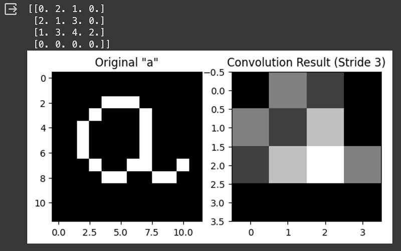
Using a stride length higher than 3 is not recommended, as our kernel size is 3x3, so a stride of 4 will make the kernel miss some image positions.
Now, what happens if instead of a 3x3 filter, we use a 4x4 filter? We can test by creating a new filter and perform the convolution step again:
# Convolution filter
filter_a = np.array([
    [1, 1, 1, 1],
    [1, 1, 1, 1],
    [1, 1, 1, 1],
    [1, 1, 1, 1]
])

# Initialize the result matrix
result = np.zeros((matrix_a.shape[0] - filter_a.shape[0] + 1, matrix_a.shape[1] - filter_a.shape[1] + 1))

for i in range(matrix_a.shape[0] - filter_a.shape[0] + 1):
    for j in range(matrix_a.shape[1] - filter_a.shape[1] + 1):
        result[i, j] = np.sum(matrix_a[i:i+filter_a.shape[0], j:j+filter_a.shape[1]] * filter_a)

# Print the result
print(result)

# Display the original 'a' and the result
plt.subplot(1, 2, 1)
plt.imshow(matrix_a, cmap='gray')
plt.title('Original "a"')

plt.subplot(1, 2, 2)
plt.imshow(result, cmap='gray')
plt.title('Convolution Result')

plt.show()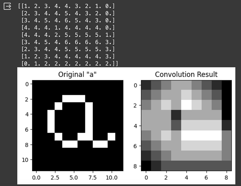
It is possible to see that a bigger kernel cannot detect as much detail as a smaller 3x3 kernel. But what if we use an even bigger 5x5 kernel?
# Convolution filter
filter_a = np.array([
    [1, 1, 1, 1, 1],
    [1, 1, 1, 1, 1],
    [1, 1, 1, 1, 1],
    [1, 1, 1, 1, 1],
    [1, 1, 1, 1, 1]
])

# Initialize the result matrix
result = np.zeros((matrix_a.shape[0] - filter_a.shape[0] + 1, matrix_a.shape[1] - filter_a.shape[1] + 1))

for i in range(matrix_a.shape[0] - filter_a.shape[0] + 1):
    for j in range(matrix_a.shape[1] - filter_a.shape[1] + 1):
        result[i, j] = np.sum(matrix_a[i:i+filter_a.shape[0], j:j+filter_a.shape[1]] * filter_a)

# Print the result
print(result)

# Display the original 'a' and the result
plt.subplot(1, 2, 1)
plt.imshow(matrix_a, cmap='gray')
plt.title('Original "a"')

plt.subplot(1, 2, 2)
plt.imshow(result, cmap='gray')
plt.title('Convolution Result')

plt.show()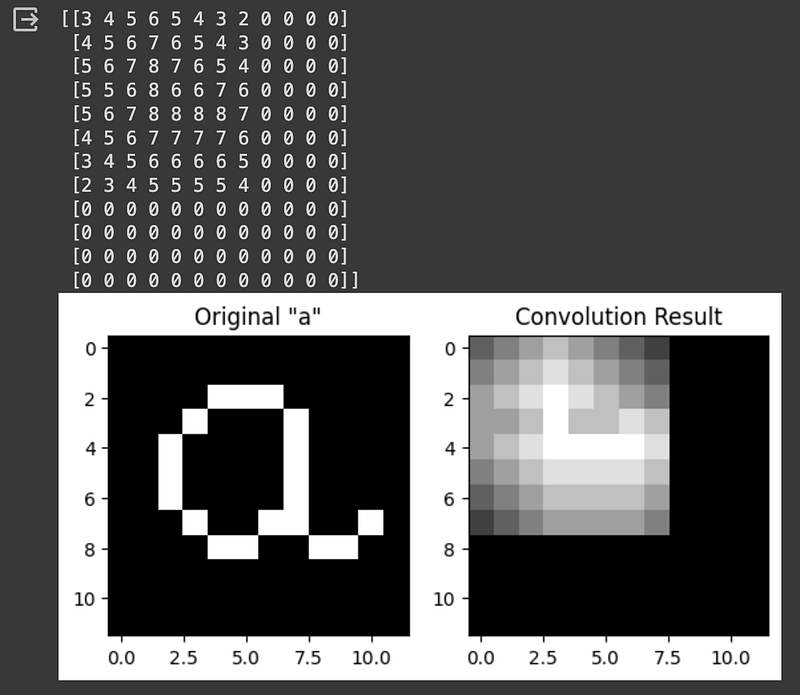
We can see that the level of detail keeps degrading as we use a bigger kernel. Remember that smaller kernels can detect more detail, while bigger kernels are more advantageous to capture features that are present in every part of the image. We can also increase the stride length if we use a bigger kernel:
# Perform convolution with stride of 2
# Initialize the result matrix
result = np.zeros((matrix_a.shape[0] - filter_a.shape[0] + 1, matrix_a.shape[1] - filter_a.shape[1] + 1))

stride_length = 2
result = np.zeros((1 + (matrix_a.shape[0] - filter_a.shape[0]) // stride_length,
                   1 + (matrix_a.shape[1] - filter_a.shape[1]) // stride_length))

for i in range(0, matrix_a.shape[0] - filter_a.shape[0] + 1, stride_length):
    for j in range(0, matrix_a.shape[1] - filter_a.shape[1] + 1, stride_length):
        result[i // stride_length, j // stride_length] = np.sum(matrix_a[i:i+filter_a.shape[0], j:j+filter_a.shape[1]] * filter_a)

# Print the result
print(result)

# Display the original 'a' and the result
plt.subplot(1, 2, 1)
plt.imshow(matrix_a, cmap='gray')
plt.title('Original "a"')

plt.subplot(1, 2, 2)
plt.imshow(result, cmap='gray')
plt.title(f'Convolution Result (Stride {stride_length})')

plt.show()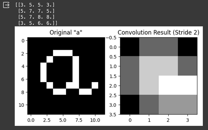
Conversely, if we use a smaller kernel, more detail is conserved in the output. See what happens with a 2x2 kernel:
# Convolution filter
filter_a = np.array([
    [1, 1],
    [1, 1]
])

# Initialize the result matrix
result = np.zeros((matrix_a.shape[0] - filter_a.shape[0] + 1, matrix_a.shape[1] - filter_a.shape[1] + 1))

for i in range(matrix_a.shape[0] - filter_a.shape[0] + 1):
    for j in range(matrix_a.shape[1] - filter_a.shape[1] + 1):
        result[i, j] = np.sum(matrix_a[i:i+filter_a.shape[0], j:j+filter_a.shape[1]] * filter_a)

# Print the result
print(result)

# Display the original 'a' and the result
plt.subplot(1, 2, 1)
plt.imshow(matrix_a, cmap='gray')
plt.title('Original "a"')

plt.subplot(1, 2, 2)
plt.imshow(result, cmap='gray')
plt.title('Convolution Result')

plt.show()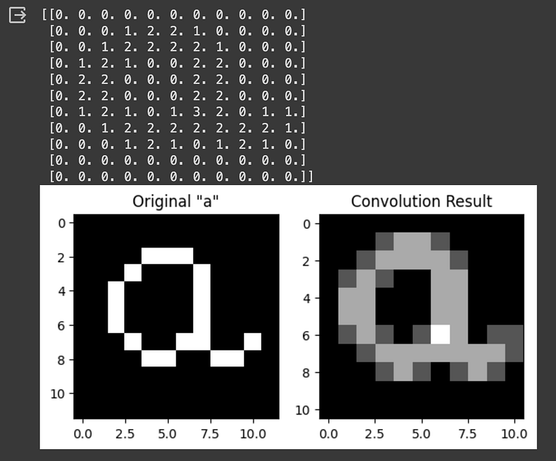
We can see that detail is preserved even when we increase the stride length:
# Perform convolution with stride of 2
# Initialize the result matrix
result = np.zeros((matrix_a.shape[0] - filter_a.shape[0] + 1, matrix_a.shape[1] - filter_a.shape[1] + 1))

stride_length = 2
result = np.zeros((1 + (matrix_a.shape[0] - filter_a.shape[0]) // stride_length,
                   1 + (matrix_a.shape[1] - filter_a.shape[1]) // stride_length))

for i in range(0, matrix_a.shape[0] - filter_a.shape[0] + 1, stride_length):
    for j in range(0, matrix_a.shape[1] - filter_a.shape[1] + 1, stride_length):
        result[i // stride_length, j // stride_length] = np.sum(matrix_a[i:i+filter_a.shape[0], j:j+filter_a.shape[1]] * filter_a)

# Print the result
print(result)

# Display the original 'a' and the result
plt.subplot(1, 2, 1)
plt.imshow(matrix_a, cmap='gray')
plt.title('Original "a"')

plt.subplot(1, 2, 2)
plt.imshow(result, cmap='gray')
plt.title(f'Convolution Result (Stride {stride_length})')

plt.show()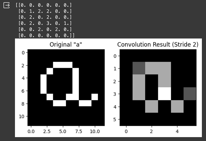
Finally, we can also simulate a pooling layer. In the previous example, we have only summed up the obtained values in each kernel, but we can apply MaxPooling or AveragePooling too. Let's see an example of MaxPooling:
#Max Pooling
# Initialize the result matrix
result = np.zeros((matrix_a.shape[0] - filter_a.shape[0] + 1, matrix_a.shape[1] - filter_a.shape[1] + 1))

for i in range(matrix_a.shape[0] - filter_a.shape[0] + 1):
    for j in range(matrix_a.shape[1] - filter_a.shape[1] + 1):
        submatrix = matrix_a[i:i+filter_a.shape[0], j:j+filter_a.shape[1]]* filter_a
        result[i, j] = np.max(submatrix)


# Print the result
print(result)

# Display the original 'a' and the result
plt.subplot(1, 2, 1)
plt.imshow(matrix_a, cmap='gray')
plt.title('Original "a"')

plt.subplot(1, 2, 2)
plt.imshow(result, cmap='gray')
plt.title(f'Convolution Result')

plt.show()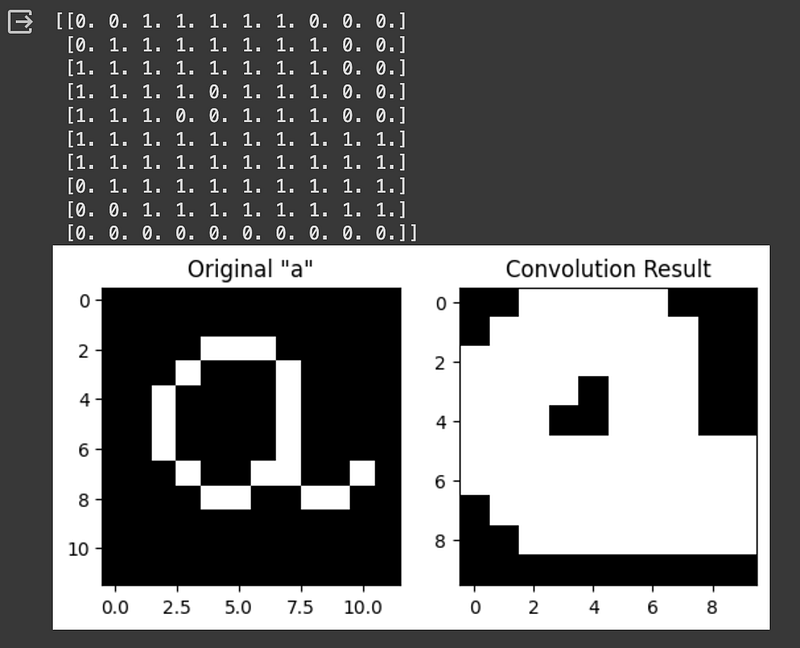
Another example of Average Pooling:
#Average Pooling
# Initialize the result matrix
result = np.zeros((matrix_a.shape[0] - filter_a.shape[0] + 1, matrix_a.shape[1] - filter_a.shape[1] + 1))

# Compute the mean without using filter_a
for i in range(result.shape[0]):
    for j in range(result.shape[1]):
        submatrix = matrix_a[i:i+filter_a.shape[0], j:j+filter_a.shape[1]] * filter_a
        result[i, j] = np.mean(submatrix)


# Print the result
print(result)

# Display the original 'a' and the result
plt.subplot(1, 2, 1)
plt.imshow(matrix_a, cmap='gray')
plt.title('Original "a"')

plt.subplot(1, 2, 2)
plt.imshow(result, cmap='gray')
plt.title(f'Convolution Result')

plt.show()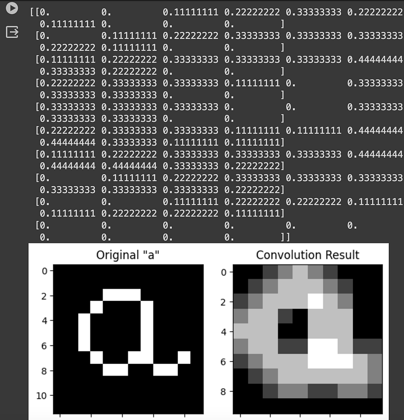
Thank you for reading! Don’t forget to subscribe to receive notifications about my future publications.
If: you liked this article, don’t forget to follow me and thus receive all updates about new publications.
Else If: you want to read more on the topic, you can buy my book “Data-Driven Decisions: A Practical Introduction to Machine Learning” which will give you all the information you need to start with Machine Learning. It will cost you only a coffee, and give me a small tip!
Else: Thank you!

