Algorithms: Insertion Sort in JavaScript

A brief look at insertion sort written in JavaScript, including checking the loop invariant and analyzing the run time.

Implementing Insertion Sort

Insertion sort is a very simple algorithm that works best for data that is already mostly sorted. Before getting started, it is always a good idea have a visualization of how the algorithm functions. You can refer to the video at the top of the post to get a sense for how insertion sort works. I recommend using the scrubber to slide through the animation one frame at a time and watch how the indices change.

The basic idea is that we select one element at a time and then search for the correct place to insert it. Hence the name, insertion sort. This results in the array having two parts — the sorted part of the array and the elements that have yet to be sorted. Some like to picture this as two different arrays — one with all of the unsorted elements and a new one that is entirely sorted. However, picturing it as one array is more true to how the code works.

Let’s take a look at the code block and and then discuss it.

The code for insertion sort has two indices, i and j. i tracks our outer loop and represents the current element we are sorting. It starts at 1 instead of 0 because when we only have one element in our newly sorted array, there is nothing to sort. Therefore, we start at the second element and compare it against the first. The second index, j, starts at i-1 and iterates from right-to-left until it finds the correct location to place the element. Along the way, we move each element over by one to make room for the new element being sorted.

And that’s all there is to it! If you are just interested in the implementation, then you do not need to read any further. But if you would like to know what makes this implementation correct, then please continue!

Checking the Loop Invariant Conditions

In order to know for sure that our algorithm is working correctly and not just accidentally giving us the correct output for the given input, we can establish a set of conditions that must be true at the beginning of the algorithm, the end of it, and every step in-between. This set of conditions is called the loop invariant and must hold true after each loop iteration.

The loop invariant is not something that is always the same. It depends entirely on the implementation of the algorithm and is something we must determine as the designer of the algorithm. In our case, we iterate through the array one at a time, and then search right-to-left for the correct place to insert it. This results in the left part of the array, up to the current index, always being a sorted permutation of the elements originally found in that slice of the array. In other words…

The loop invariant for insertion sort states that all elements up to the current index, A[0..index], make up a sorted permutation of the elements originally found in A[0..index] before we began sorting.

To check these conditions, we need a function that can be called from within the loop that takes in as arguments:

1. The newly sorted array
2. The original input
3. The current index.

Once we have that, we will slice the arrays from 0 to the current index and run our checks. The first check is that all elements in the new array are contained within the old array and second, that they are all in order.

If we call this function before, during, and after our loop and it passes without any errors, we can be confident that our algorithm is working properly. Modifying our code to include this check would look like this…

const insertionSort = (nums) => {
  checkLoopInvariant(nums, input, 0)
  for (let i = 1; i < nums.length; i++) {
    ...
    checkLoopInvariant(nums, input, i)
    while (j >= 0 && nums[j] > tmp) {
      ...
    }
    nums[j+1] = tmp
  }
  checkLoopInvariant(nums, input, nums.length)
  return nums
}

For a visual example, consider the state of our array after when the index is 2, so it has sorted 3 elements.

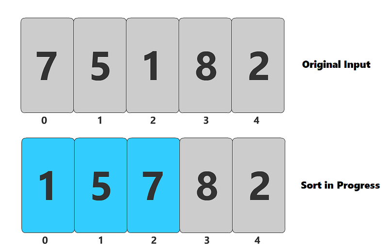
As you can see, we have processed 3 elements and those first 3 elements are in order. You can also see that the first 3 numbers of the sorted array are the same as the first 3 numbers in the original input, just in a different order. Thus, the loop invariant is maintained.

Analyzing the Run Time

The last thing we are going to be looking at with insertion sort is the run time. Performing a true run time analysis involves a lot of math and you can find yourself in the weeds pretty quickly. If you are interested in that type of analysis, please refer to Cormen’s Introduction to Algorithms, 3rd Edition. For the purposes of this post, however, we are only going to be performing a worst-case analysis.

The worst-case scenario for insertion sort is that the input array is in reverse-sorted order. This means that for every element that we iterate over, we will end up having to iterate backwards over every element we have already sorted to find the correct insertion point. The outer loop can be represented as a summation from 2 to n (where n is the size of the input), and each iteration has to perform i-1 operates as it iterates from i-1 down to zero.

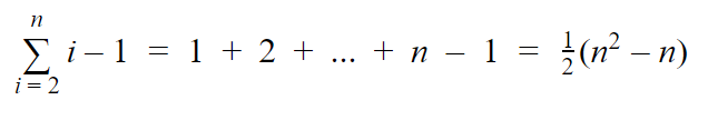
The proof for that summation is out of the scope of this post. I honestly just plugged it into Wolfram Alpha. Just to compare that to the best-case scenario, in which the elements are already sorted, so each iteration is constant time…

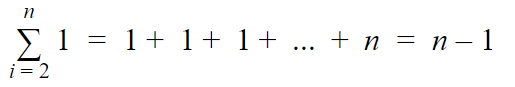
In terms of big-O notation, the worst-case scenario is Ɵ(n²) and the best-case is Ɵ(n). We always take the worst-case result though, so the algorithm as a whole is Ɵ(n²).

Summary

Insertion sort works best when the input array is already mostly sorted. A good application for this is inserting a new element into an already sorted data-store. Even though you will likely never have to write your own sorting algorithms, and other sorts, such as merge sortand quick sort, are faster, I believe it’s fun to analyze algorithms in this way.

If you have any questions, or if I got anything incorrect, please don’t hesitate to leave a comment below! :)