InfoGAN: Interpretable Representation Learning to Distangle Data Unsupervised

Unlike conditional GAN, which requires explicit class labels, InfoGAN can capture latent representations unsupervised. With the learnt latent variable, we can manipulate/control the outputs. The method introduces Information Maximizing to the standard GAN network.

1. Introduction
2. The math (about entropy and variational inference)
3. The implementation in PyTorch

1. Introduction

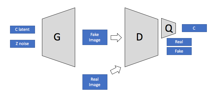
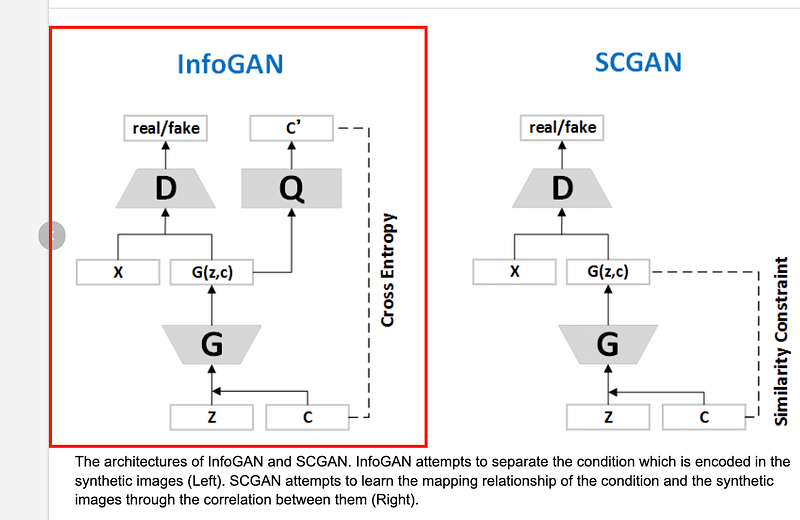
InfoGAN was introduced by Chen et al.[1] in 2016. On top of GAN having a generator and a discriminator, there is an auxiliary network called the Q-network. The Q-network is responsible for predicting the latent code from the generated data. The key idea of InfoGAN is to maximize the mutual information between the latent code and the generated data.

The latent code is divided into three parts: noise, categorical variables, and continuous variables. The noise is the random input to the generator, as in the standard GAN. Categorical variables can represent discrete attributes (e.g., digit class in the MNIST dataset). Continuous variables can represent continuous attributes (e.g., rotation or thickness of a digit in the MNIST dataset). The generator inputs these three parts of the latent code and produces the generated data.

During training, the Q-network learns to predict the categorical and continuous variables from the generated data while the generator tries to generate data that helps the Q-network make accurate predictions. The mutual information between the latent code and the generated data is maximized, resulting in a more interpretable and meaningful latent space.

2. The math

(1) Information theory

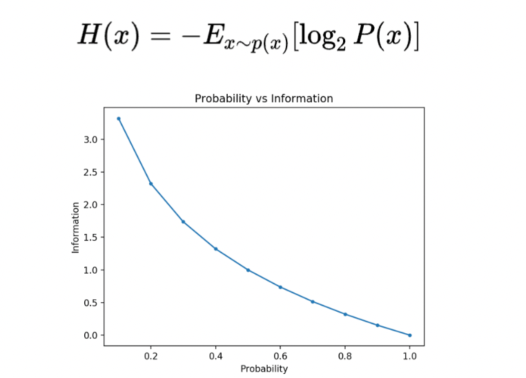
The concept of mutual information is from information theory. In the machine learning context, the information theory is used to quantify the similarity between probability distributions. Unlikely or surprising events have more information; this is why the news always reports exaggerated events.

To quantify how much information there is in a message, called entropy, is calculated using probability. It measures the amount of uncertainty in the entire PDF.

And the mutual information between the random variables X and Y, I(X, Y), measures the amount of information learned about X from Y:

• I(X,Y) = H(X) — H(X|Y) = H(Y) — H(Y|X)
• if H(X|Y) = 0, X is determined by Y since no more information is added given Y. So, I(X,Y) = H(X), meaning those two variables are dependent.
• if H(X|Y) = H(X), X is independent because Y can’t provide any information about X. So, I(X, Y) =0, X and Y are independent

(2) The loss function

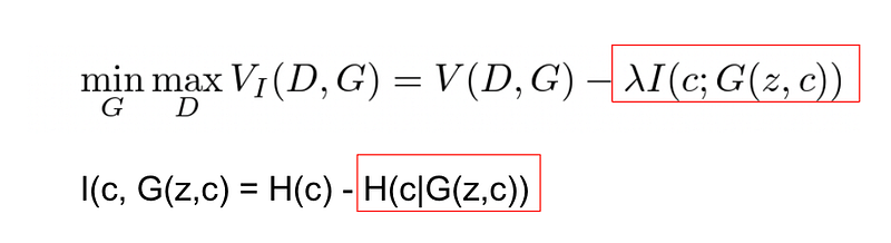
Where V(D, G) is the regular GAN loss function. The objective of this loss function involves maximising the latter regularization term, which means minimizing H(c|G(z,c)) (if H(X|Y) = 0, X is determined by Y).

(3) The variational inference trick

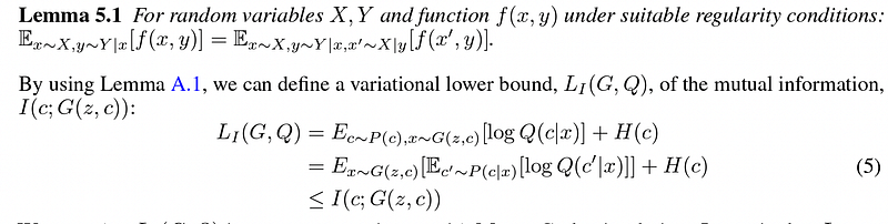
However, the mutual information I(c; G(z, c)) is hard to maximize as it requires access to the posterior P(c|x). But a lower bound can be obtained using an auxiliary distribution Q(c|x) to approximate P(c|x). This is called the variational lower bound.

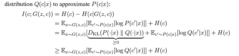
Since it still requires getting access to P(c|x), the author uses the Lemma to get around the problem.

This video clearly explains those concepts with detailed formula derivations [2], which is highly recommended.

3. The implementation in PyTorch

In the InfoGAN structure, only a new Q network needed to add to the basic/standard GAN network. It is observed that the model always converges faster than normal GAN objectives, and hence InfoGAN essentially comes for free with GAN.

Training on the MNIST dataset, the Q network will output (1) the discrete, which digit to generate, (2) the continuous, the angle.

Networks:

import torch
import torch.nn as nn
import torch.nn.functional as F

class Generator(nn.Module):
    def __init__(self):
        super().__init__()

        self.tconv1 = nn.ConvTranspose2d(74, 1024, 1, 1, bias=False)
        self.bn1 = nn.BatchNorm2d(1024)

        self.tconv2 = nn.ConvTranspose2d(1024, 128, 7, 1, bias=False)
        self.bn2 = nn.BatchNorm2d(128)

        self.tconv3 = nn.ConvTranspose2d(128, 64, 4, 2, padding=1, bias=False)
        self.bn3 = nn.BatchNorm2d(64)

        self.tconv4 = nn.ConvTranspose2d(64, 1, 4, 2, padding=1, bias=False)

    def forward(self, x):
        x = F.relu(self.bn1(self.tconv1(x)))
        x = F.relu(self.bn2(self.tconv2(x)))
        x = F.relu(self.bn3(self.tconv3(x)))

        img = torch.sigmoid(self.tconv4(x))

        return img

class Discriminator(nn.Module):
    def __init__(self):
        super().__init__()

        self.conv1 = nn.Conv2d(1, 64, 4, 2, 1)

        self.conv2 = nn.Conv2d(64, 128, 4, 2, 1, bias=False)
        self.bn2 = nn.BatchNorm2d(128)

        self.conv3 = nn.Conv2d(128, 1024, 7, bias=False)
        self.bn3 = nn.BatchNorm2d(1024)

    def forward(self, x):
        x = F.leaky_relu(self.conv1(x), 0.1, inplace=True)
        x = F.leaky_relu(self.bn2(self.conv2(x)), 0.1, inplace=True)
        x = F.leaky_relu(self.bn3(self.conv3(x)), 0.1, inplace=True)

        return x

class DHead(nn.Module):
    def __init__(self):
        super().__init__()

        self.conv = nn.Conv2d(1024, 1, 1)

    def forward(self, x):
        output = torch.sigmoid(self.conv(x))

        return output

class QHead(nn.Module):
    def __init__(self):
        super().__init__()

        self.conv1 = nn.Conv2d(1024, 128, 1, bias=False)
        self.bn1 = nn.BatchNorm2d(128)

        self.conv_disc = nn.Conv2d(128, 10, 1)
        self.conv_mu = nn.Conv2d(128, 2, 1)
        self.conv_var = nn.Conv2d(128, 2, 1)

    def forward(self, x):
        x = F.leaky_relu(self.bn1(self.conv1(x)), 0.1, inplace=True)

        disc_logits = self.conv_disc(x).squeeze()

        mu = self.conv_mu(x).squeeze()
        var = torch.exp(self.conv_var(x).squeeze())

        return disc_logits, mu, var

# Initialise the network.
netG = Generator().to(device)
discriminator = Discriminator().to(device)
netD = DHead().to(device)
netQ = QHead().to(device)

The loss function includes this Q network loss:

        # Updating Generator and QHead
        optimG.zero_grad()

        # Fake data treated as real.
        output = discriminator(fake_data)
        label.fill_(real_label)
        probs_fake = netD(output).view(-1)
        gen_loss = criterionD(probs_fake, label.float())

        q_logits, q_mu, q_var = netQ(output)
        target = torch.LongTensor(idx).to(device)
        # Calculating loss for discrete latent code.
        dis_loss = 0
        for j in range(params['num_dis_c']):
            dis_loss += criterionQ_dis(q_logits[:, j*10 : j*10 + 10], target[j])

        # Calculating loss for continuous latent code.
        con_loss = 0
        if (params['num_con_c'] != 0):
            con_loss = criterionQ_con(noise[:, params['num_z']+ params['num_dis_c']*params['dis_c_dim'] : ].view(-1, params['num_con_c']), q_mu, q_var)*0.1

        # Net loss for generator.
        G_loss = gen_loss + dis_loss + con_loss
        # Calculate gradients.
        G_loss.backward()
        # Update parameters.
        optimG.step()

Check the complete Colab code here, which refers to this GitHub repo.

If you liked posts like this, you might also like a Medium membership. It’s only $5 a month, but it will give you unlimited access to articles while supporting your favourite writers. If you sign up using this link, I’ll earn a small commission. Thanks!

References:

[1]Chen, X., Duan, Y., Houthooft, R., Schulman, J., Sutskever, I., & Abbeel, P. (2016). Infogan: Interpretable representation learning by information maximizing generative adversarial nets. Advances in neural information processing systems, 29.

[2]https://www.youtube.com/watch?v=ohRtxx30Ev8&list=PLdxQ7SoCLQANQ9fQcJ0wnnTzkFsJHlWEj&index=41

https://www.youtube.com/watch?v=qIJez258ri8&list=PLdxQ7SoCLQANQ9fQcJ0wnnTzkFsJHlWEj&index=41

BECOME a WRITER at MLearning.ai