In-depth Exploration of Garbage Collector (GC)

Algorithms, trade-offs, and real-life applications

Introduction

In traditional programming languages like C or C++, developers are responsible for explicitly allocating and deallocating memory for objects and data structures.

However, manual memory management can be error-prone, leading to bugs such as memory leaks (where allocated memory is not released) or dangling pointers (where pointers reference memory that has already been deallocated). These issues can result in unstable or insecure software.

Garbage collection addresses these challenges by automating the memory management process. Instead of requiring developers to manually allocate and deallocate memory, garbage collectors automatically identify and reclaim memory that is no longer reachable or referenced by the program.

Garbage collection algorithms vary in complexity and implementation, and different programming languages and runtime environments may use different garbage collection strategies.

While garbage collection offers significant benefits, such as automatic memory management and prevention of memory-related bugs, it also introduces overhead in terms of CPU and memory usage.

This article aims to explore different Garbage Collector algorithms, examining their internal workings, benefits, and limitations.

This will assist us in choosing the suitable algorithm and configuration, allowing us to write the code with greater efficiency.

I hope that this article will serve as a valuable reference for future studies.

Brace yourself as we set out on this adventure; here is the plan I suggest: · A tidbit of history ∘ Running Program’s Memory ∘ Garbage Collector’s emergence ∘ Garbage Collector overview · Mark-Sweep ∘ Operating principle and algorithm ∘ Real use cases · Copying ∘ Operating principle and algorithm ∘ Real use cases · Mark-Compact ∘ Operating principle and algorithm ∘ Real use cases · Generational ∘ Operating principle and algorithm ∘ Real use cases · Garbage-first (G1) ∘ Operating principle and algorithm ∘ Real use cases · Z ∘ Operating principle and algorithm ∘ Real use cases · Shenandoah ∘ Operating principle and algorithm ∘ Real use cases · Epsilon ∘ Operating principle and algorithm ∘ Real use cases · Comparing garbage collectors algorithms · Conclusion

Here we go!

A tidbit of history

Running Program’s Memory

A typical memory layout of a running program can be as follows:

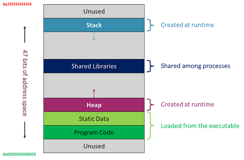
For the duration of the program, Static memory is used to store global variables or those declared with the static keyword.

The Stack is a designated memory area where computer programs temporarily hold data. It is a contiguous memory block that stores data during function calls and clears it once the functions conclude.

Stack memory follows the Last-In-First-Out (LIFO) principle, meaning the latest item placed on the stack will be the first to be removed.

Upon a function call, the program generates a new element known as a Stack Frame, which is then pushed onto the stack for that particular function call.

A Stack Frame consists of:

• Local variables of the function.
• Parameters passed to the function.
• The return address, which directs the program where to resume execution after the function finishes.
• Additional elements, like the base pointer of the preceding frame.

Once the function completes execution, its Stack Frame is removed, and control is transferred back to the return address indicated within the frame.

Keep in mind that Stack memory has a limited capacity, and when it’s exhausted, a Stack Overflow occurs, leading to program failure. Consequently, the Stack is not ideal for storing large data volumes.

Additionally, the Stack does not allow memory blocks to be resized once they are allocated. For example, If we allocate too little memory for an array on the Stack, it won’t be able to be resized like with dynamically allocated memory.

These factors led to the invention of Heap memory.

A Heap is an area of computer memory designated for dynamic memory allocation. Contrary to Stack memory, which is managed automatically, Heap memory requires manual management using methods like malloc to allocate memory and free to deallocate it.

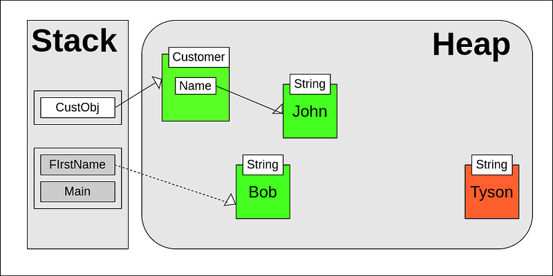
Objects on the Heap are accessed through references, which serve as pointers to these objects. Objects are instantiated within the Heap space, while Stack memory holds the references to them:

The Heap is commonly used in situations where:

• The memory needed for a data structure, like an array or an object, cannot be determined until runtime (dynamic allocation).
• Data must be retained beyond the duration of a single function call.
• There is a potential need to resize the allocated memory at some point in the future.

In the upcoming steps, the focus will be on managing Heap memory.

Garbage Collector’s emergence

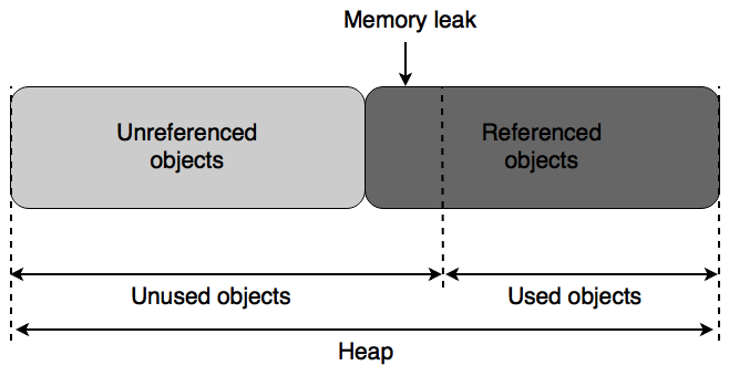
Memory occupied by Heap objects can be reclaimed either manually through explicit deallocation, using operations like C’s free or C++’s delete, or automatically by the runtime system via Reference Counting or Garbage Collection.

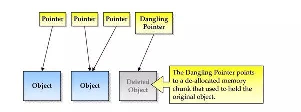
The manual memory management can result in two primary types of programming errors:

🔴 The first is the premature freeing of memory while references to it still exist, resulting in what is known as a dangling pointer.

🔴 The second is the potential failure to release an object no longer needed by the program, resulting in a memory leak.

These issues become even more complex in concurrent programming, where multiple threads may reference an object simultaneously.

Thus, it was necessary to evaluate and reorganize ideas, which resulted in the creation of automatic memory management.

To make things simpler, automatic memory management can be viewed as a refactoring of manual memory management:

☑️ Memory management is centralized in a single tool, the Garbage Collector, which is runtime-controlled (generally by a Virtual Machine).

☑️ The Garbage Collector’s approach to memory management has simplified the process of manual memory release, making the code easier to read and maintain.

☑️ Memory debugging and profiling become more efficient.

☑️ The upgrade to the Garbage Collector and the automatic memory management algorithms has become scalable, universal, and efficient.

What secrets does the Garbage Collector hold? Let’s look!

Garbage Collector overview

A Garbage Collector (GC) is a background and periodically-triggered program that automatically frees up memory taken by objects that are no longer in use, thereby making this memory available for the application’s future needs.

In what way does the GC identify unused objects?

The Garbage Collector (GC) identifies unused objects by locating those that are no longer referenced by any part of the running program. If an object does not have any active references, it is considered dead and eligible for collection, freeing up memory.

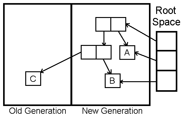
The Heap can be referenced by not only local variables, but also global and static variables, thread stacks (objects referenced by the execution stacks of threads), and the constant pool (which stores the constant values a program uses).

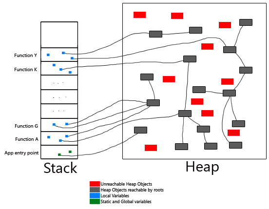
Any pointer (reference) that holds an object in the Heap but does not reside in the Heap itself can be termed as a root. Garbage Collection requires these roots to determine whether an object is live. If an object is directly or transitively reachable by any of the roots, then it is not considered garbage. If it is not reachable, it is deemed garbage and needs to be collected.

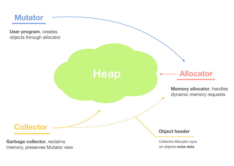
Managed memory systems consist of a mutator and a garbage collector that operate within the Heap:

• The mutator is our program (application) that modifies objects in Heap.
• The mutator claims memory on the Heap through the allocator, while the collector is responsible for reclaiming the memory space on the Heap.
• The memory allocator and the garbage collector collaborate to manage the memory space of a program’s Heap.

The essential characteristics of a garbage collector include:

• minimal overall execution time (throughput).
• optimal space usage (memory overhead).
• minimal pause time (esp. real time tasks).
• improved locality for mutator.
• scalability.

The above characteristics are influenced by the various algorithms used for garbage collectors, which differ in their approaches, optimizations, and trade-offs.

In the next sections, we will examine these different algorithms to determine their strengths, limitations, and potential real-world uses.

Here we go!

Mark-Sweep

Operating principle and algorithm

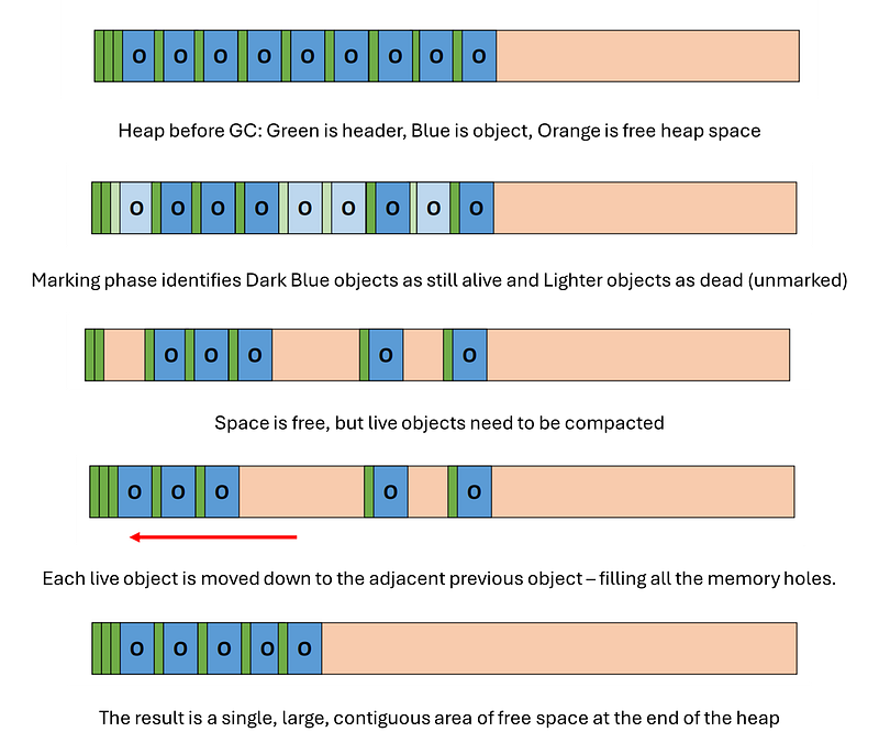
Mark-Sweep ‘naïve’ algorithm, which was introduced by John McCarthy in 1960 for Lisp, is based on a ‘stop-the-world’ mechanism. When a program requests memory and none is available, the program is stopped, and a full garbage collection is performed to free up space.

Mark-Sweep GC’s operation can be summed up in these stages:

1️⃣ The first step is to extract and prepare the root list. The roots could be local variables, global variables, static variables, or variables referenced in the thread stack.

2️⃣ Once we identified all the roots, we proceed with the mark phase. The mark phase entails a Depth-first search (DFS) traversal of a root node, with the goal of labeling all nodes reachable from the root node as ‘live’.

Many garbage collector algorithms employ at the heart of the collection procedure a tracing routine, which marks every object that is reachable from an initial set of roots. The tracing routine typically performs a graph traversal, employing a mark-stack which contains a set of objects that were visited but whose children have not yet been scanned. The tracing procedure repeatedly pops an object from the mark-stack, marks its children, and inserts each previously unmarked child to the mark-stack. The order by which objects are inserted and removed from the mark-stack determines the tracing order. The most common tracing orders are DFS (depthfirst search) for a LIFO mark-stack, and BFS (breadth-first search) for a mark-stack that works as a FIFO queue.

Data Structure Aware Garbage Collector

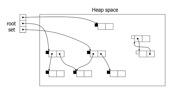
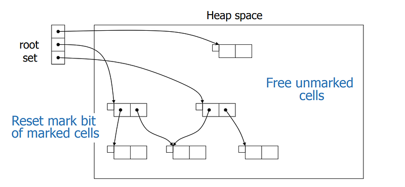
3️⃣ The nodes left unmarked are garbage, and hence during the sweep phase, the GC iterates through all the objects and frees the unmarked objects. It also resets the marked objects to prepare them for the next cycle.

A basic Mark-Sweep algorithm can be as follows:

//Marking
Add each object referenced by the root set to Unscanned and set its reached-bit to 1;
while(Unscanned != empty set){
     remove some object o from Unscanned;
     for(each object o' referenced in o){
         if(o' is unreached; i.e, reached-bit is 0){
              set the reached-bit of o' to 1;
            place o' in Unscanned;
         }
     }
}

//Sweeping
Free = empty set;
for(each chunk of memory o in heap){
    if(o is unreached, i.e, its reached-bit is 0) add o to Free;
    else set reached-bit of o to 0;
}

Mark-Sweep GC has an advantage: since objects do not move during GC, there is no need to update their pointers. However, it also has several disadvantages:

• Its sweeping phase is costly due to the difficulty in locating unreachable objects without scanning the entire Heap.
• The program’s execution must be stopped to perform garbage collection, resulting in significant performance issues.
• The accumulation of unused memory across the Heap can cause memory fragmentation, making it unusable for new objects.

Clearly, the Mark-Sweep GC is not suitable for real-time systems.

Let’s see how this algorithm is really implemented and used.

Real use cases

The algorithm applied in its ‘naïve’ version can be found in these applications:

1️⃣ uLisp:

The type of garbage collector used in uLisp is called mark and sweep. First, markobject() marks all the objects that are still accessible. Then sweep() builds a new freelist out of the unmarked objects, and unmarks the marked objects.

uLisp — Garbage collection

2️⃣ Ruby’s earlier versions:

The first version of Ruby already has a GC using Mark and Sweep (M&S) algorithm. M&S is one of the most simple GC algorithms which consists of two phases: (1) Mark: traverse all living objects and mark as “living object”. (2) Sweep: garbage collect unmarked objects as they are unused.

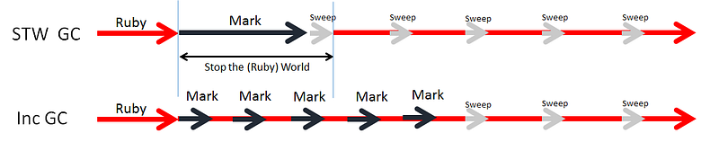
While M&S algorithm is simple and works well, there are several problems. The most important concerns are “throughput” and “pause time”. GC slows down your Ruby program because of GC overhead. In other words, low throughput increases total execution time of your application. Each GC stops your Ruby application. Long pause time affects UI/UX on interactive web applications. Ruby 2.1 introduced generational garbage collection to overcome “throughput” issue.

Incremental Garbage Collection in Ruby 2.2 | Heroku

Moreover, there are improved versions of the ‘naïve’ algorithm that can be found:

1️⃣ Incremental Mark-Sweep algorithm:

➖ Ruby 2.2:

Incremental GC algorithm splits a GC execution process into several fine-grained processes and interleaves GC processes and Ruby processes. Instead of one long pause, incremental garbage collection will issue many shorter pauses over a period of time. The total pause time is the same (or a bit longer because of overhead to use incremental GC), but each individual pause is much shorter. This allows the performance to be much more consistent. Incremental Garbage Collection in Ruby 2.2 | Heroku

➖ OCaml:

The major heap is typically much larger than the minor heap and can scale to gigabytes in size. It is cleaned via a mark-and-sweep garbage collection algorithm that operates in several phases […] The mark-and-sweep phases run incrementally over slices of the heap to avoid pausing the application for long periods of time, and also precede each slice with a fast minor collection. Only the compaction phase touches all the memory in one go, and is a relatively rare operation. Understanding the Garbage Collector — Real World OCaml

➖ Mozilla SpiderMonkey:

SpiderMonkey has a mark-sweep garbage collection (GC) with incremental marking mode, generational collection, and compaction. Much of the GC work is performed on helper threads. Garbage collection (realityripple.com)

2️⃣ Concurrent Mark-Sweep (CMS) algorithm:

The Concurrent Mark Sweep (CMS) collector is designed for applications that prefer shorter garbage collection pauses and that can afford to share processor resources with the garbage collector while the application is running. Concurrent Mark Sweep (CMS) Collector (oracle.com)

The concurrent mark sweep collector (concurrent mark-sweep collector, concurrent collector or CMS) was a mark-and-sweep garbage collector in the Oracle HotSpot Java virtual machine (JVM) available since version 1.4.1. It was deprecated on version 9 and removed on version 14, so from Java 15 it is no longer available. Concurrent mark sweep collector — Wikipedia

FYI, Java has replaced the Concurrent Mark Sweep (CMS) with Z Garbage Collector (ZGC) and Shenandoah collector that we will see in the next sections.

Copying

Operating principle and algorithm

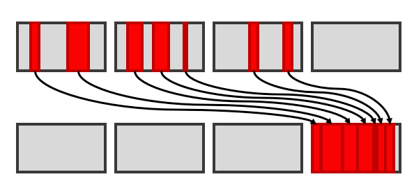
The idea of Copying Garbage Collection is to split the Heap in two semi-spaces of equal size: the ‘from-space’ and the ‘to-space’:

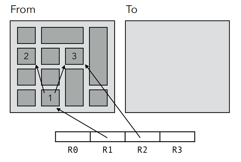
1️⃣ Memory is allocated in ‘from-space’, while ‘to-space’ is left empty.

2️⃣ When ‘from-space’ is full, all reachable objects in ‘from-space’ are copied to ‘to-space’, and pointers to them are updated accordingly.

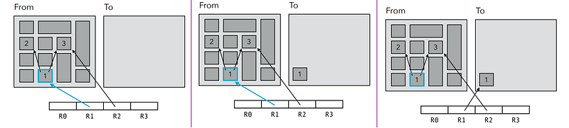
⛔ Before copying an object, it is necessary to verify whether it has been previously copied. If it has, the object should not be copied again; instead, the existing copy should be utilized. This verification is done by placing a ‘forwarding pointer’ in the ‘from-space’ object once it’s been copied.

3️⃣ Finally, the role of the two spaces is exchanged, and the program resumed.

✔️ In a copying garbage collector, memory allocation occurs linearly in ‘from-space’, eliminating the need for a free list or a search for a free block. All that’s required is to mark the boundary between the allocated and free areas of ‘from-space’ with just one pointer.

✔️Furthermore, allocation in a copying garbage collector is very quick, almost as fast as stack allocation.

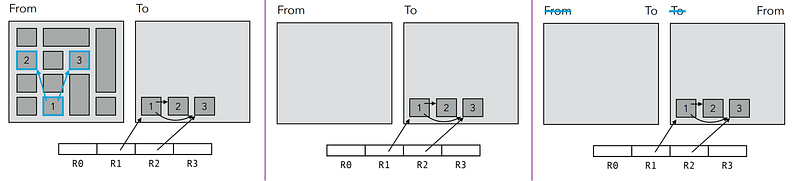
The ‘naïve’ copying garbage collection (GC) algorithm performs a Depth-First traversal of the reachable graph, which can cause a stack overflow when implemented recursively.

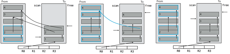
In contrast, Cheney’s copying GC algorithm is an efficient technique that conducts a Breadth-First traversal of the reachable graph and requires only a single pointer as additional state:

✳️ In any Breadth-First traversal, it’s necessary to keep track of the set of nodes that have been visited, but whose children have not yet been explored.

Extra memory, usually a queue, is needed to keep track of the child nodes that were encountered but not yet explored. Breadth-first search — Wikipedia

✳️ Cheney’s algorithm fundamentally uses the ‘to-space’ to store this set of nodes, which is denoted by a single pointer named ‘scan’.

✳️ This pointer divides the ‘to-space’ into two sections: one for nodes whose children have been visited and another for those whose children are yet to be visited.

➕ The advantages of using copying garbage collection instead of mark-and-sweep are the elimination of external fragmentation, rapid allocation, and avoidance of dead object traversal.

➕ A key characteristic of Cheney’s algorithm is that it never touches any object that needs to be freed; it only follows pointers from live objects to live objects.

➖ However, the disadvantages include the consumption of twice as much virtual memory, the necessity for accurate pointer identification, and the potential high cost of copying.

I came across this pseudo-code that implements the Cheney’s algorithm.

Let’s see how this algorithm is really implemented and used.

Real use cases

1️⃣ Ocaml:

To garbage-collect the minor heap, OCaml uses copying collection to move all live blocks in the minor heap to the major heap. This takes work proportional to the number of live blocks in the minor heap, which is typically small according to the generational hypothesis. In general, the garbage collector stops the world (that is, halts the application) while it runs, which is why it’s so important that it complete quickly to let the application resume running with minimal interruption.

Understanding the Garbage Collector — Real World OCaml

2️⃣ LISP:

Fenichel and Yochelson have described how performance will degrade over time in LISP systems utilizing virtual memory. Their solution, copying garbage collection, as further modified by Cheney, was widely adopted in modern LISP systems; but its performance was limited by the need to scan a potentially large root set, and to move from one area to the other, on each garbage collection, all the structures maintained through a computation.

A Lifetime-Based Garbage Collector for LISP Systems on General-Purpose Computers. (dtic.mil)

3️⃣ Chicken (Scheme implementation):

The design used is a copying garbage collector originally devised by C. J. Cheney, which copies all live continuations and other live objects to the heap.

Chicken (Scheme implementation) — Wikipedia

Our exploration of the realm of Copying Garbage Collection concludes at this juncture; let us now venture into a new algorithm!

Mark-Compact

Operating principle and algorithm

I will begin with this piece:

Mark–compact algorithms can be regarded as a combination of the mark–sweep algorithm and Cheney’s copying algorithm. First, reachable objects are marked, then a compacting step relocates the reachable (marked) objects towards the beginning of the heap area. Mark–compact algorithm — Wikipedia

The Mark-compact algorithms go through various stages during operation:

1️⃣ It starts with the marking phase, where live data is identified.

2️⃣ Next, the live data is compacted by relocating objects and updating the pointer values of all live references to objects that have moved.

There are various ways in which compacting can be carried out, whether by preserving the original order or disregarding it. The following are the different methods:

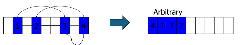
1️⃣ Arbitrary: no logical or spatial order is maintained.

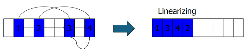
2️⃣ Linearizing: objects are moved and then ordered based on logical relations, i.e. objects that point to one another are moved into adjacent positions.

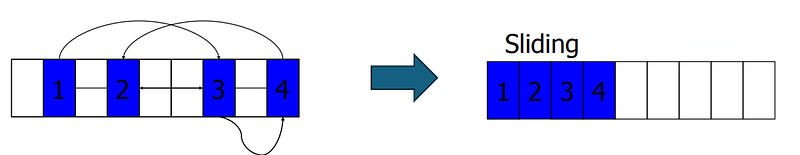
3️⃣ Sliding: maintaining the original order of allocation.

Let’s see how this algorithm is really implemented and used.

Real use cases

There are five well-known compact algorithms:

• Two-finger algorithm (Saunders — 1974): it’s not really used in practice due to performance issues.
• Lisp 2 algorithm.
• Jonkers’ threaded algorithm (1979).
• SUN’s parallel algorithm (Flood-Detlefs-Shavit-Zhang — 2001).
• IBM’s parallel algorithm (Abuaiadh-Ossia-Petrank-Silbershtein — 2004).
• The Compressor (Kermany-Petrank — 2006).

Algorithms can be categorized as follows:

• Uni-processor compaction includes Two-finger, Lisp2, and Jonkers’ threaded.
• Parallel compaction encompasses Sun’s compaction, IBM’s compaction, and Compressor (parallel and concurrent, delayed…).

Here is a table summarizing the characteristics of the Uni-processor compaction algorithms:

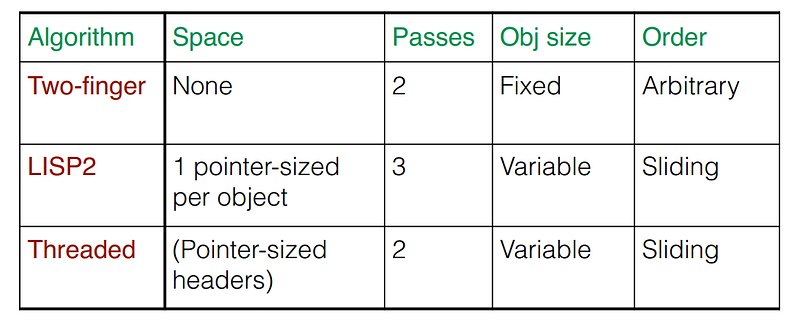
This table compares the performance of Jonkers’ threaded algorithm, IBM’s Parallel Compaction algorithm that is restricted to a single thread, and IBM’s Parallel Compaction algorithm that is fully parallel (the time is in milliseconds):

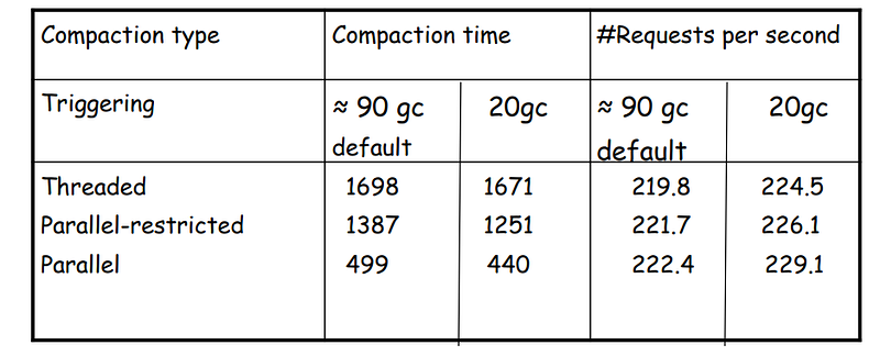
IBM’s Parallel Compaction algorithm remains efficient even when restricted to a single thread, offering notable speedup and high-quality compaction.

Let’s move forward with more advanced algorithms!

Generational

Operating principle and algorithm

Generational garbage collection involves segregating objects into generations according to their age and prioritizing the collection of younger generations over older ones.

1️⃣ The Young Generation is where all new objects are allocated and aged.

2️⃣ When the young generation fills up, this causes a minor garbage collection. A young generation full of dead objects is collected very quickly.

🚩 All minor garbage collections are ‘stop-the-world (STW)’ events.

3️⃣ Some of the surviving objects are promoted to the Old Generation, based on a Promotion Policy.

4️⃣ The Old Generation is used to store long surviving objects. Typically, a threshold is set for young generation object and when that age is met, the object gets moved to the old generation.

5️⃣ When the Old generation is full, a major collection is performed to collect memory in that generation and all the younger ones.

6️⃣ Also, a threshold is set for Young Generation objects, and when that threshold (i.e. the number of times an object has been copied) is met, the objects are moved to the old generation.

🚩Major garbage collection are also Stop the World events.

✔️ Most generational collectors manage Younger Generations by copying: original copying collector, parallel copying collector or parallel scavenge collector.

✔️ Managing old generations can be achieved through a Mark-Sweep algorithm, Concurrent Collector, or Incremental Collector.

Let’s review the advantages and disadvantages from what we’ve seen:

➕ Generational GC tends to reduce GC pause times since only the youngest generation, which is also the smallest, is collected most of the time.

➕ In copying GCs, the use of generations also avoids copying long-lived objects over and over.

➖ As live objects can be in different generation spaces in this scheme, the issue of inter-generational pointers (e.g. a pointer from an older generation to a younger one) rises.

➖ Since old generations are not collected as often as young ones, it is possible for dead old objects to prevent the collection of dead young objects. This problem is called Nepotism.

Let’s see how this algorithm is really implemented and used.

Real use cases

1️⃣ Python:

Standard CPython’s garbage collector has two components, the reference counting collector and the generational garbage collector, known as gc module. — Garbage collection in Python: things you need to know | Artem Golubin (rushter.com)

In order to limit the time each garbage collection takes, the GC implementation for the default build uses a popular optimization: generations. The main idea behind this concept is the assumption that most objects have a very short lifespan and can thus be collected soon after their creation. This has proven to be very close to the reality of many Python programs as many temporary objects are created and destroyed very quickly. To take advantage of this fact, all container objects are segregated into three spaces/generations. Every new object starts in the first generation (generation 0). The previous algorithm is executed only over the objects of a particular generation and if an object survives a collection of its generation it will be moved to the next one (generation 1), where it will be surveyed for collection less often. If the same object survives another GC round in this new generation (generation 1) it will be moved to the last generation (generation 2) where it will be surveyed the least often. — Garbage collector design (python.org)

2️⃣ Ruby:

Back to the crux of the point here: as of Ruby 2.1, Ruby introduced Generational GC which takes advantage of the weak generational hypothesis. It concentrates more frequent garbage collection efforts on young, newer objects. Ruby’s garbage collector actually has two different types of garbage collection: major GCs and minor GCs. Minor GCs happen more frequently, and mostly look at young objects. (There’s an edge case here which we’ll cover in a bit.) Major GCs happen less frequently and look at all objects. Minor GCs are faster than major GCs because they’re looking through fewer objects. — Ruby Garbage Collection Deep Dive: Generational Garbage Collection | Jemma Issroff

3️⃣ V8’s garbage collection:

V8 uses a generational garbage collector with the Javascript heap split into a small young generation for newly allocated objects and a large old generation for long living objects. Since most objects die young, this generational strategy enables the garbage collector to perform regular, short garbage collections in the smaller young generation (known as scavenges), without having to trace objects in the old generation. The young generation uses a semi-space (copying) allocation strategy, where new objects are initially allocated in the young generation’s active semi-space. Once that semi-space becomes full, a scavenge operation will move live objects to the other semi-space. Objects which have been moved once already are promoted to the old generation and are considered to be long-living. Once the live objects have been moved, the new semi-space becomes active and any remaining dead objects in the old semi-space are discarded. The old generation uses a mark-and-sweep collector (incrementally mark live objects in many small steps) with several optimizations to improve latency and memory consumption. — Getting garbage collection for free · V8

4️⃣ Java serial collector:

The Serial GC is the simplest Java GC algorithm. It is the default collector on single-core 32-bit machines. […] The serial collector is a generational garbage collector that uses an evacuating, also known as mark and copy, collector for the young generation and a mark-sweep-compact (MSC) collector for the old generation. The young generation collector is called Serial, while the old generation collector is called Serial (MSC). However, the serial collector is impractical for most modern server-side applications. […] The parallel collector is the default garbage collector on 64-bit machines with two or more CPUs (up to Java 8). It is similar to serial collectors in that it is a generational collector, but it uses multiple threads to perform garbage collection. The parallel collector collects both the young and old generations using multiple threads. The parallel collector uses a mark-and-copy collector called ParallelScavenge for the young generation and a mark-sweep-compact collector called ParallelOld for the old generation collection, similar to the serial collector. However, the main difference is the use of multiple threads in the parallel collector. — Understanding JVM Garbage Collection — Part 6 (Serial and Parallel Collector) — A Bias For Action

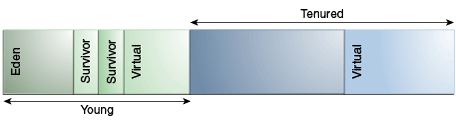
The young generation consists of eden and two survivor spaces. Most objects are initially allocated in eden. One survivor space is empty at any time, and serves as the destination of any live objects in eden; the other survivor space is the destination during the next copying collection. Objects are copied between survivor spaces in this way until they are old enough to be tenured (copied to the tenured generation). — Generations (oracle.com)

I am fascinated by the variety of algorithms and reflections made. Let’s further the enchantment with the subsequent sections that delve into more modern and sophisticated GCs!

Garbage-first (G1)

Operating principle and algorithm

Garbage-First (G1) is a garbage collection algorithm introduced by Sun Microsystems for use in Java Virtual Machines (JVMs).

It is a generational, regionalized, incremental, parallel, mostly concurrent, stop-the-world, and evacuating (compacting) garbage collector.

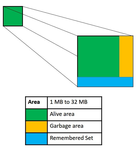
🔵 A regionalized garbage collector indicates that the Heap is divided into multiple regions, each of equal size:

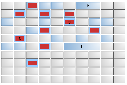
🔵 Every region is composed of different components:

• Space: the space allocated for each region can vary from 1MB to 32MB, depending on the maximum Heap size.
• Alive: a portion of the objects within a region will still be in use.
• Garbage : some objects in the region are no longer needed and can be classified as garbage.
• RSet: the Remembered Set serves as a form of metadata that helps keep track of which objects are alive and which are no longer needed. This data aids the JVM in calculating the percentage of live objects in a region at any given time (Liveness % = Live Size / Region Size).

🔵 The Eden, Survivor, and Old regions are not required to be contiguous like the older garbage collectors (logical set of regions):

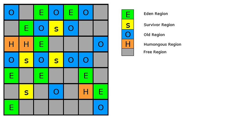
🔵 Eden regions (‘E’) and Survivor regions (‘S’) are part of the Young Generation.

🔵 An application always allocates objects into the Young Generation specifically in Eden regions, with the exception of humongous (‘H’) objects (objects that span multiple regions) that are directly allocated as belonging to the Old Generation.

🔵 The G1 collector alternates between two phases: the young-only phase and the space-reclamation phase.

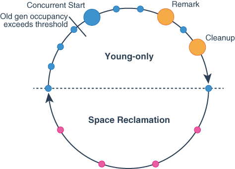
1️⃣ Young-only GC is responsible for promoting objects from Eden to Survivor regions or Survivor regions to Old generation regions. Young-only events are considered to be stop-the-world (i.e. STW) events.

2️⃣ G1 collector performs below phases as part of Young-only GC:

• Initial Mark: starts the marking process along with regular young-only collection. Concurrent marking determines all the live objects in old generation regions (it is not a stop-the-world event).
• Remark: finalizes marking by performing global reference processing and class unloading. Reclaims completely empty regions and cleans up internal data structures (this is a stop-the-world event).
• Cleanup: determines if a space-reclamation mixed collection is necessary (this is a stop-the-world event).

3️⃣ The space-reclamation phase involves several Mixed collections that not only target young generation regions but also evacuate live objects from selected old generation regions.

4️⃣ The space-reclamation phase concludes when G1 concludes that further evacuation of old generation regions would not result in a significant amount of free space to justify the effort.

5️⃣ After space-reclamation, the collection cycle restarts with another young-only phase.

6️⃣ If the application runs out of memory when gathering liveness information, G1 will perform an in-place stop-the-world full Heap compaction (Full GC), as a precautionary measure, similar to other collectors.

🔵 Based on what we have seen, here are some advantages and disadvantages of using G1:

➕ Advantages:

• Predictable pause times.
• Region-based collection.
• Adaptive sizing.
• Compaction.
• Soft real-time performance.

➖ Disadvantages:

• Initial marking pause.
• Increased CPU overhead.
• Less maturity compared to other collectors.
• Heap fragmentation.
• Configuration complexity.

In summary, Garbage-First (G1) provides considerable benefits such as predictable pause times and effective memory management. However, it may not be ideal for every application and often necessitates meticulous tuning for optimal performance.

The Garbage-First (G1) collector is a server-style garbage collector, targeted for multi-processor machines with large memories. It meets garbage collection (GC) pause time goals with a high probability, while achieving high throughput. — Getting Started with the G1 Garbage Collector (oracle.com)

Real use cases

The Garbage-First (G1) algorithm was created for Java Virtual Machines (JVMs) and is commonly used in programming languages that operate on the JVM, mainly Java. Any Java application that makes use of the JVM’s garbage collection function can potentially see improvements with the G1 garbage collector.

It is important to note that G1 is not limited to the Java language itself, but rather to the JVM runtime environment. Other languages like Kotlin, Scala, Groovy, and Clojure that can be run on the JVM can also make use of the G1 garbage collector when running on the JVM.

Let’s maintain our momentum, and in the following section, we will delve into the workings of another modern garbage collector: Z. Onward!

Z

Operating principle and algorithm

The Z Garbage Collector (ZGC) is a high-performance garbage collector specifically designed to handle large memory Heaps, such as those in the terabyte range.

The ZGC has two categories: Non-generational ZGC and Generational ZGC. The non-generational ZGC is available in production since Java 15, while the generational ZGC is part of Java 21.

And I found this draft about deprecating non-generational ZGC in future release:

Deprecate non-generational ZGC, with the intent to remove it in a future release. Switch Generational ZGC to be the default ZGC mode, and deprecate the ZGenerational flag. JEP draft: Deprecate Non-Generational ZGC (openjdk.org)

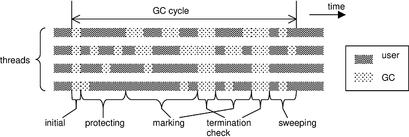
ZGC manages nearly all garbage collection processes concurrently:

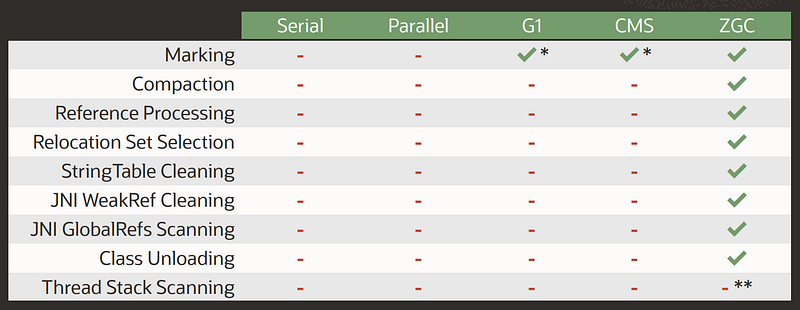
The ZGC operating cycle consists of 3 phases. Each one starts with a ‘safe-point’ synchronization point involving a pause of all application threads, aka STW “Stop-The-World”. Apart from these 3 points, all operations are carried out concurrently with the rest of the application:

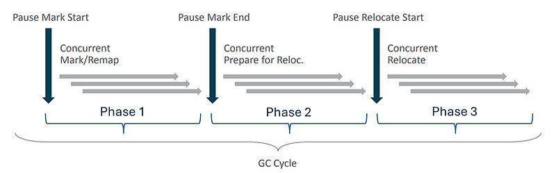
These pauses are always below the millisecond:

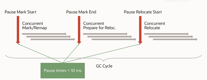
1️⃣ Phase 1: The cycle begins with a synchronization pause (STW1) which allows:

• threads to identify the right “color” to use (colored pointers).
• to create memory pages (ZPages).
• to ensure that all “GC roots” are valid (have the right colour), correcting them if necessary (Load Barriers)

The subsequent concurrent phase of Mark/Remap consists of traversing the object graph to identify the objects that are candidates for collection.

2️⃣ Phase 2: The STW2 pause marks the end of the marking phase. Concurrent treatments allow for the identification of memory regions that need compacting.

3️⃣ Phase 3: After again identifying the correct color in STW3, the objects are moved concurrently to compact the memory, which completes the cycle.

Let’s delve into the details of the various keywords we’ve previously encountered:

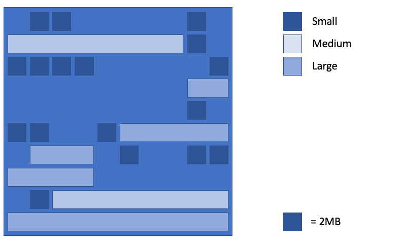
✳️ ZPages: ZGC segments the Heap memory into regions known as ZPages, which are categorized as small, medium, and large:

• Small (2 MiB — object size up to 256 KiB).
• Medium (32 MiB — object size up to 4 MiB).
• Large (4+ MiB — object size > 4 MiB).

Small and medium-sized pages can hold multiple objects, whereas large pages are limited to a single object. This restriction helps prevent the movement of large objects, which would require copying extensive memory ranges and could result in significant latency.

✳️ Compaction and Relocation: the Heap objects are constantly compacted to address the problem of progressive memory fragmentation and guarantee the fast allocation of new objects.

During the lifecycle, compactable pages are identified (marked) in Phase 2 (typically those with the fewest objects), and then all objects residing on those pages are relocated in Phase 3. Once a page is devoid of any objects, its memory can be reclaimed.

In order to perform these relocation operations concurrently, ZGC maintains routing tables. These are stored off-heap and optimized for fast reading, at the expense of additional memory cost.

✳️ Colored Pointers: The goal is to store information about an object’s life cycle within its pointer. This is a key element that allows many operations to be performed concurrently.

4 bits are dedicated to storing these meta-data:

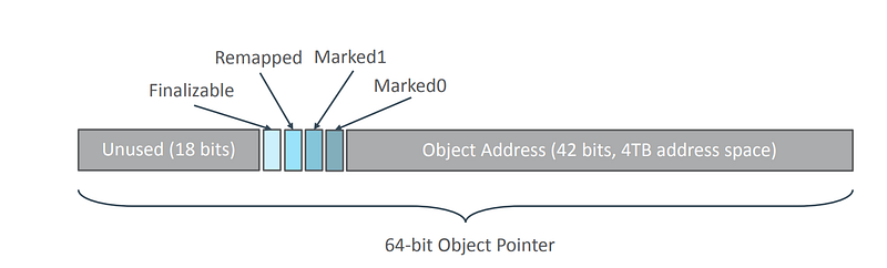
The ‘color’ of a pointer is determined by the state of the 3 meta-bits Marked0 (M0), Marked1 (M1) and Remapped (R):

• M0 and M1 are used to tag objects to collect.
• Remapped indicates that the reference has been relocated.

🚩 Only one of these three bits can have value 1. Consequently, three colors were obtained: M0 (100), M1 (010), and R (001).

A color is either ‘good’ or ‘bad’, and this is determined globally at several stages of the life cycle:

• Newly instantiated objects are marked with the correct color.
• The ZGC cycle begins with a brief stop-the-world pause (STW 1), during which the correct color is identified by alternately changing the values of bits M0 and M1. Thus, if M0 is the correct color in one cycle, M1 will be the correct color in the following cycle.
• During the next concurrent phase, known as Concurrent Mark/Remap, if the garbage collector encounters a pointer that is incorrectly colored, it will update the pointer to the correct address and assign the appropriate color.
• In the last synchronization point of the cycle (STW 3) R becomes the correct color.

✳️ Heap Multi-Mapping: Multi-memory mapping allows multiple virtual addresses to point to the same physical address. Thus, two pointers whose virtual address differs only by their metadata point to the same physical address.

The ZGC needs this technique since ZGC can move the physical location of an object in Heap memory while the application is running. With multi-mapping, the physical location of an object is mapped to three views in virtual memory, corresponding to each of the pointer’s potential ‘colors’:

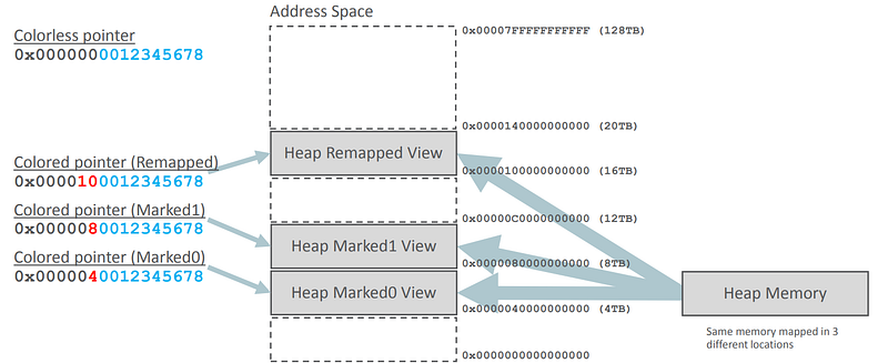
This enables a load barrier to identify an object that has been relocated since the last synchronization point.

✳️ Load barriers: are small segments of code that the JIT compiler injects at strategic points, specifically when an object reference is being loaded from the Heap.

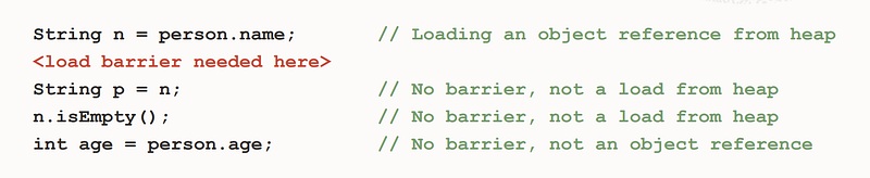
Thus, thanks to load barriers, an object can be moved at any time without the pointers referencing it being updated. Load barriers intercept the reading of its pointers and correct them. This ensures that at any time, when a pointer is loaded, it points to the right object while GC and application threads are running concurrently.

In computing, a memory barrier, also known as a membar, memory fence or fence instruction, is a type of barrier instruction that causes a central processing unit (CPU) or compiler to enforce an ordering constraint on memory operations issued before and after the barrier instruction. This typically means that operations issued prior to the barrier are guaranteed to be performed before operations issued after the barrier. — Memory barrier — Wikipedia

Real use cases

Z Garbage Collector (ZGC) is primarily used with Java applications that run on the Java Virtual Machine (JVM). Therefore, any programming language that compiles to Java bytecode and runs on the JVM can potentially utilize ZGC. The most prominent language in this category is Java itself.

However, it’s worth noting that other languages besides Java can also run on the JVM, including Kotlin, Scala, Groovy, Clojure, and JRuby, among others. As long as these languages leverage the JVM for execution, they can benefit from the features and optimizations provided by ZGC if configured to do so.

In summary, while ZGC is primarily associated with Java due to its integration with the JVM, it can also be used with other JVM-based languages.

Let’s maintain the rhythm and proceed to the next algorithm!

Shenandoah

Operating principle and algorithm

Shenandoah is primarily developed by Red Hat and is available as an experimental feature in OpenJDK starting from Java 12. It is actively developed and supported by the community.

✔️ While both Shenandoah and ZGC prioritize minimizing pause times through concurrent garbage collection, Shenandoah is designed to be fully concurrent, aiming to avoid STW pauses altogether. ZGC, while highly concurrent in its approach, may still have brief STW pauses in certain phases of garbage collection.

✔️ While both Shenandoah and ZGC use a segmented approach to manage the Heap, they differ in the granularity of their segmentation. Shenandoah uses larger regions, while ZGC uses smaller ZPages.

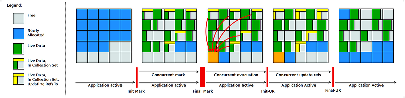
✔️ Shenandoah operates in several phases, including initial marking, concurrent marking, concurrent evacuation (concurrent copying of live objects), and concurrent cleanup:

✔️ Shenandoah mainly employs a concurrent evacuation method, whereas ZGC utilizes a combination of techniques, such as concurrent marking, evacuation (relocating live objects), and compaction (minimizing fragmentation).

✔️ While both Shenandoah and ZGC use specialized pointer techniques to maintain consistency during garbage collection, they employ different mechanisms — Shenandoah uses Brooks pointers, while ZGC uses Colored pointers.

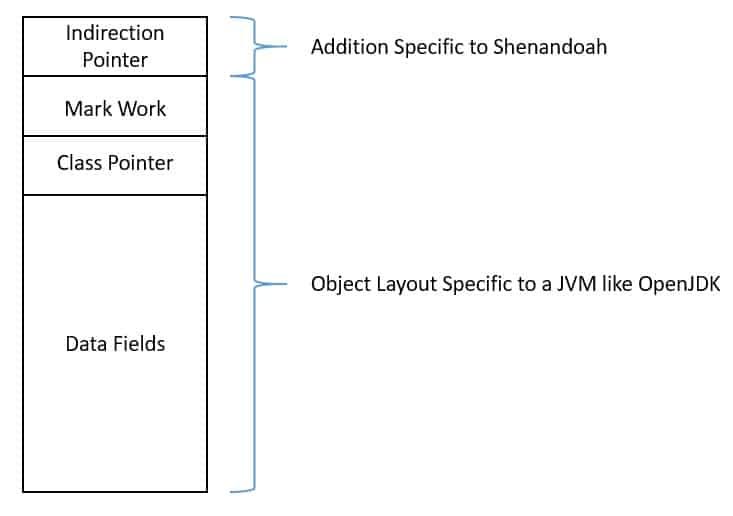
Shenandoah adds an additional word to this object layout. This serves as the indirection pointer and allows Shenandoah to move objects without updating all of the references to them. This is also known as the Brooks pointer. Experimental Garbage Collectors in the JVM | Baeldung

✔️ Both Shenandoah and ZGC rely on load barriers to ensure memory consistency and correctness during garbage collection. The load barrier intercepts reads of object references made by application threads and ensures that they observe a consistent view of the Heap, even in the presence of concurrent garbage collection operations.

💡 Shenandoah is the optimal choice for those prioritizing ultra-low latency and fully concurrent operations, particularly for large Heap sizes and dynamic workloads. Conversely, ZGC stands out as the ideal option for a proven, low-latency garbage collector that offers extensive compatibility and ease of configuration.

Real use cases

Shenandoah Garbage Collector (GC) is primarily used with Java applications running on the Java Virtual Machine (JVM). Therefore, any programming language that compiles to Java byte-code and runs on the JVM can potentially utilize Shenandoah GC. The most prominent language in this category is Java itself.

However, it’s worth noting that other languages besides Java can also run on the JVM, including Kotlin, Scala, Groovy, Clojure, and JRuby, among others. As long as these languages leverage the JVM for execution, they can benefit from the features and optimizations provided by Shenandoah GC if configured to do so.

In summary, while Shenandoah GC is primarily associated with Java due to its integration with the JVM, it can also be used with other JVM-based languages.

We are nearing the end; we just need to uncover one last GC, and then we can proceed to the comparison. Let’s go!

Epsilon

Operating principle and algorithm

Epsilon GC is a special garbage collector introduced in Java 11 as an experimental feature. Unlike traditional garbage collectors, which reclaim memory by identifying and collecting unused objects, Epsilon GC does not perform any garbage collection at all. Instead, it allows the Java Virtual Machine (JVM) to allocate memory without ever collecting garbage!

Here are some key points about Epsilon GC:

✔️ No Garbage Collection: Epsilon GC does not perform any garbage collection. It allocates memory as needed but never reclaims it. This makes it useful for scenarios where garbage collection overhead is not a concern, such as short-lived applications or applications that manage memory manually.

✔️ For Performance Testing: Epsilon GC is primarily intended for performance testing and bench-marking purposes. By eliminating the overhead of garbage collection, developers can focus solely on application performance without interference from garbage collection pauses.

✔️ Not Suitable for Production: Epsilon GC is not suitable for production environments where memory management and garbage collection are essential for application stability and performance. It is meant for testing and experimental purposes only.

⛔ Epsilon GC provides a unique option for performance testing and experimentation by completely eliminating garbage collection overhead. However, it is not intended for production use and may have limited applicability depending on the specific requirements of the application.

Real use cases

Epsilon GC is a garbage collector specifically designed for the Java Virtual Machine (JVM). Therefore, it is not directly associated with any programming language other than Java. Any Java application that runs on a JVM with support for Epsilon GC can potentially utilize it.

It’s time to sum it up!

Comparing garbage collectors algorithms

Comparing garbage collection algorithms involves evaluating various factors such as pause times, throughput, scalability, memory overhead, and suitability for specific application scenarios.

1️⃣ Serial or single-threaded Garbage Collectors:

• Pause Times: Typically has longer pause times as it stops all application threads during garbage collection.
• Throughput: Generally lower throughput compared to concurrent garbage collectors.
• Scalability: May not scale well with large Heap sizes or multi-threaded applications.
• Memory Overhead: Typically has lower memory overhead compared to other collectors.
• Suitability: Suitable for small to medium-sized applications or applications where pause times are not critical.

2️⃣ Parallel Garbage Collector:

• Pause Times: Reduced pause times compared to serial collector as it uses multiple threads for garbage collection.
• Throughput: Higher throughput compared to serial collector due to parallelism.
• Scalability: Scales better with multi-core processors and larger Heap sizes.
• Memory Overhead: Generally higher memory overhead compared to serial collector due to additional threads.
• Suitability: Suitable for mid-sized applications where throughput is important but pause times are not critical.

3️⃣ Concurrent Mark-Sweep (CMS) Garbage Collector:

• Pause Times: Designed to minimize pause times by performing most of the garbage collection work concurrently with the application threads.
• Throughput: Moderate throughput but may suffer from fragmentation issues.
• Scalability: May not scale well with very large Heap sizes or highly multi-threaded applications.
• Memory Overhead: Moderate memory overhead.
• Suitability: Suitable for applications with medium-sized Heaps and latency-sensitive requirements.

4️⃣ Garbage-First (G1) Garbage Collector:

• Pause Times: Intended to provide low-pause-time behavior by dividing the Heap into regions and performing garbage collection incrementally.
• Throughput: Good throughput for most applications, especially those with large Heaps.
• Scalability: Scales well with multi-core processors and large Heap sizes.
• Memory Overhead: Moderate memory overhead due to region-based management.
• Suitability: Suitable for large-scale applications where low pause times and good throughput are both important.

5️⃣ Z Garbage Collector (ZGC):

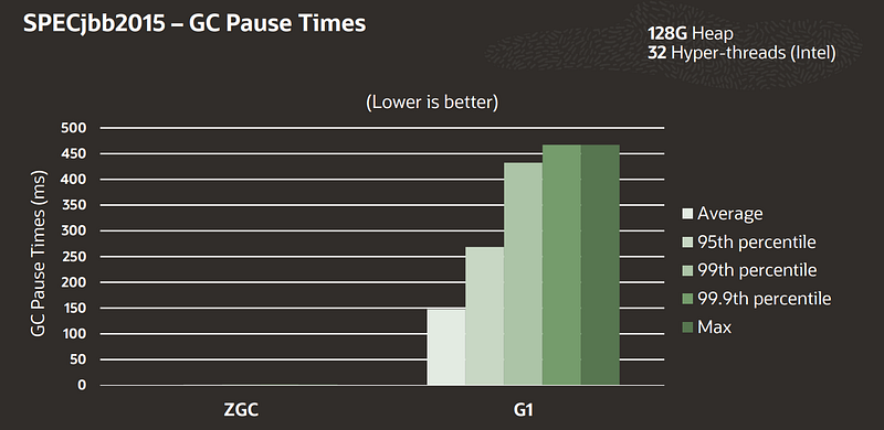
• Pause Times: Designed to provide ultra-low-latency behavior with pause times typically below 10ms, even on large Heaps.
• Throughput: Offers good throughput for most applications while prioritizing low pause times.
• Scalability: Highly scalable with support for very large Heap sizes and multi-threaded applications.
• Memory Overhead: Moderate memory overhead with the use of ZPages and other techniques.
• Suitability: Suitable for applications with strict latency requirements and large Heap sizes.

6️⃣ Shenandoah Garbage Collector:

• Pause Times: Aims for ultra-low-latency behavior with concurrent garbage collection, minimizing pause times even on large Heaps.
• Throughput: Offers good throughput while prioritizing low pause times.
• Scalability: Highly scalable with support for very large Heap sizes and multi-threaded applications.
• Memory Overhead: Moderate memory overhead with the use of region-based management.
• Suitability: Suitable for applications with strict latency requirements and large Heap sizes, particularly those with dynamic memory allocation patterns.

In summary, the choice of garbage collection algorithm depends on factors such as application requirements, Heap size, latency sensitivity, and available hardware resources. It’s essential to evaluate these factors carefully to select the most appropriate garbage collector for the specific use case.

Conclusion

Understanding garbage collection algorithms is essential for comprehending how memory management is conducted in programming languages and runtime environments that automate this task.

These algorithms vary in their approaches, optimizations, and trade-offs, influencing factors such as pause times, throughput, memory overhead, and scalability.

Although garbage collection offers automatic memory management and eases the process of memory allocation and deallocation for developers, it also presents certain trade-offs and challenges that must be thoughtfully considered in the design and implementation of software systems.

Finally, the classification of garbage collection as a ‘green technology’ hinges on multiple factors, such as its influence on resource use, energy consumption, system efficiency, and overall environmental sustainability. Although garbage collection may lead to more efficient use of resources and possibly decrease electronic waste, its environmental footprint must be assessed based on specific use cases and system setups.

I trust you found this journey through the Garbage Collector enlightening.

Until we meet again in a new article and a fresh adventure! ❤️

Thank you for reading my article.

Want to Connect? 
You can find me at GitHub: https://github.com/helabenkhalfallah