Implementing Mean Reversion Strategies in Algorithmic Trading

In algorithmic trading, mean reversion strategies are widely used to identify and exploit deviations from the average price of a financial asset. These strategies assume that prices will eventually revert back to their mean or average value. By taking advantage of these price movements, traders can potentially generate profits.

In this tutorial, we will explore how to implement mean reversion strategies in algorithmic trading using Python. We will start by understanding the concept of mean reversion and its relevance in trading. Then, we will dive into the implementation details, including data acquisition, strategy development and backtesting.

To follow along with this tutorial, you will need to have Python installed on your machine, as well as the following libraries: pandas, numpy, matplotlib, yfinance and mplfinance. You can install these libraries using the following command:

pip install pandas numpy matplotlib yfinance mplfinance

Data Acquisition

To implement our mean reversion strategy, we need historical price data for a financial asset. In this tutorial, we will use the yfinance library to download data directly from Yahoo Finance. Let’s start by importing the necessary libraries and downloading the data for a specific asset.

import yfinance as yf

# Define the ticker symbol for the asset
ticker = "JPM"

# Download the historical price data
data = yf.download(ticker, start="2018-01-01", end="2023-10-31")

In the code above, we import the yfinance library and specify the ticker symbol for the asset we want to analyze (in this case, JPM for JPMorgan Chase). We then use the download function to retrieve the historical price data for the specified period.

Data Exploration

Before diving into the implementation of our mean reversion strategy, let’s explore the downloaded data to get a better understanding of its structure and characteristics. We can use the head and tail functions to display the first and last few rows of the data, respectively.

print(data.head())
print(data.tail())

The output will show the first and last few rows of the data, including the date, open, high, low, close and volume columns. This information is crucial for our analysis and strategy development.

Strategy Development

Now that we have our historical price data, we can proceed with the development of our mean reversion strategy. The basic idea behind mean reversion is to identify periods when the price deviates significantly from its mean and take positions that anticipate a reversion to the mean.

To implement this strategy, we will calculate the rolling mean and standard deviation of the asset’s price. We will then generate trading signals based on the deviation from the mean. Let’s start by calculating the rolling mean and standard deviation using a specified window size.

# Calculate the rolling mean and standard deviation
window_size = 20
data["mean"] = data["Close"].rolling(window_size).mean()
data["std"] = data["Close"].rolling(window_size).std()

In the code above, we use the rolling function to calculate the rolling mean and standard deviation of the closing price over a specified window size (in this case, 20 days). We store the results in new columns named "mean" and "std" in the data DataFrame.

Next, we will generate trading signals based on the deviation from the mean. When the price crosses above the upper band (mean + k * std), we will consider it as a sell signal. Conversely, when the price crosses below the lower band (mean — k * std), we will consider it as a buy signal. Let’s define the value of k and generate the trading signals.

# Define the value of k
k = 1

# Generate the trading signals
data["signal"] = 0
data.loc[data["Close"] > data["mean"] + k * data["std"], "signal"] = -1
data.loc[data["Close"] < data["mean"] - k * data["std"], "signal"] = 1

In the code above, we define the value of k as 1, indicating that we consider a deviation of one standard deviation from the mean as significant. We then initialize a new column named “signal” with zeros and update it based on the buy and sell conditions.

Backtesting

Now that we have our trading signals, we can backtest our mean reversion strategy to evaluate its performance. Backtesting involves simulating the execution of trades based on historical data and calculating the resulting profits or losses.

To backtest our strategy, we will assume that we have an initial capital of $10,000 and allocate a fixed percentage of our capital to each trade. Let’s define the initial capital and the allocation percentage.

# Define the initial capital and allocation percentage
initial_capital = 10000
allocation = 0.1

In the code above, we define the initial capital as $10,000 and the allocation percentage as 10%. This means that we will allocate 10% of our capital to each trade.

Next, we will calculate the positions and the daily returns based on our trading signals. We will assume that we can execute trades at the closing price of each day.

# Calculate the positions and daily returns
data["position"] = allocation * data["signal"]
data["returns"] = data["position"].shift() * data["Close"].pct_change()

In the code above, we calculate the positions by multiplying the allocation percentage by the trading signals. We then calculate the daily returns by multiplying the positions by the percentage change in the closing price.

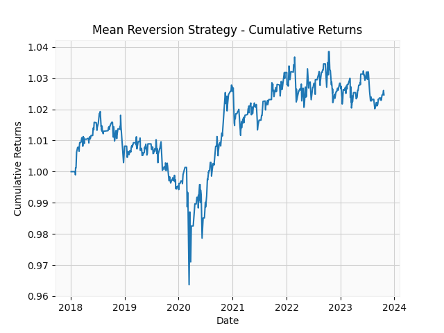
Finally, we can calculate the cumulative returns and plot them to visualize the performance of our strategy.

# Calculate the cumulative returns
data["cum_returns"] = (1 + data["returns"]).cumprod()

# Plot the cumulative returns
import matplotlib.pyplot as plt

plt.plot(data["cum_returns"])
plt.xlabel("Date")
plt.ylabel("Cumulative Returns")
plt.title("Mean Reversion Strategy - Cumulative Returns")
plt.show()

The code above calculates the cumulative returns by taking the cumulative product of the daily returns plus one. We then use matplotlib to plot the cumulative returns over time..

Conclusion

In this tutorial, we have explored how to implement mean reversion strategies in algorithmic trading using Python. We started by acquiring historical price data using the yfinance library. Then, we developed a mean reversion strategy by calculating the rolling mean and standard deviation of the asset’s price and generating trading signals based on the deviation from the mean. Finally, we backtested our strategy and evaluated its performance using cumulative returns.

Mean reversion strategies can be a powerful tool in algorithmic trading, but they require careful analysis and testing. It is important to consider factors such as transaction costs, market conditions and risk management when implementing and evaluating these strategies.

Remember to experiment with different parameters, such as the window size and the deviation threshold, to find the optimal settings for your specific trading goals. Additionally, consider incorporating other technical indicators or fundamental analysis to enhance the performance of your strategy.