Implementing a Simple Mean Reverting Pairs Trading Algorithm in the Quantconnect platform (Part 1)

Learn how to implement and backtest a Mean Reverting strategy from the book “Algorithmic Trading: Winning Strategies and Their Rationale” using the Quantconnect framework.

Update

For information about the course Introduction to Python for Scientists (available on YouTube) and other articles like this, please visit my website cordmaur.carrd.co.

Introduction

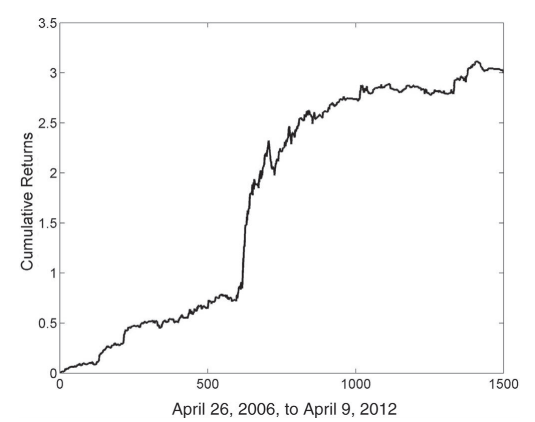
Hi! In my last story “Understanding and Implementing Kalman Filter for Pairs Trading” [1] I’ve used an example from the book Algorithmic Trading: Winning Strategies and Their Rationale [2] to illustrate the use of a Pairs Trading strategy using the Kalman Filter with the EWA (Australia’s ETF) and EWC (Canada’s ETF) pair. However, in the mentioned post, I’ve focused on the hedge ratio (relation between the two assets) and didn’t show the strategy’s performance, and that was intentional. In the Algorithmic Trading book, Ernest Chan presents an outstanding 26,2% of annualized return (APR) and a Sharpe ratio of 2.4 for this strategy from 2006 to 2012 (Figure 1).

Too good to be true?

I have implemented the Chan’s strategy in Python (the original code is in MatLab) and achieved similar results. However (remember that “the devil is in the details”), when we take a closer look at the backtest, we can notice a number of assumptions that don’t seem very realistic in a live trading environment. For example, no transaction costs or slippage are modeled, it considers that the portfolio is fully invested throughout the test, etc. Additionally, the parameters have been inferred using the same data from the backtest, incurring in the so-called look-ahead bias. Chan explains that these omissions were intended to keep source codes simpler to understand but he also raises a warning:

“I urge readers to undertake the arduous task of cleaning up such pitfalls when implementing their own backtests of these prototype strategies.”

With that in mind, I’ve decided to backtest these strategies as close as possible to reality, and that’s where Quantconnect comes in.

The Quantconnect framework

There are some ready-to-use packages to backtest a trading strategy in Python. Two good examples are Zipline and Backtrader but there are posts listing many others. Some quants even write their own code for it. The problem is that these approaches share the same shortcoming: getting good quality data.

Good quality historical data is usually charged and normally free data is provided only in a daily basis. That’s where Quantconnect comes in handy.

Quantconnect (Figure 2) is an algorithm trading framework with tons of free data to be accessed by the trading algorithms with up to minute resolution. It has also connection to different brokers so it is simple to pass from backtest to live without code adaptation. Besides that, it models brokerage transactions costs and slippage to simulate how the orders would be executed in “real” life.

So, I’ve decided to accept Chan’s “arduous” task of cleaning the pitfalls, rewriting the strategies in the Quantconnect framework, and would like to share with you the results in this new series of posts.

Linear Mean Reversion Strategy

The first strategy we are going to implement is the linear mean reversion. It assumes a constant ratio between the assets, that can be derived from a linear regression and the resulting portfolio will use the linear coefficient as the asset’s weights. To make it more clear, I will review some of the basics of cointegration and use the Quantconnect’s research environment to access the historical data.

Cointegration

In a mean reversion strategy, we assume that our series is stationary (i.e. it returns to its mean value). The problem with this assumption is that usually the stocks (and indices, and ETFs, etc.) are not stationary or mean reverting. However if we can make a combination of assets (considering some weights) and this combination is mean reverting, we will be able to trade this “combination”, and that’s the idea behind the cointegration. To exemplify, let’s use a Jupyter Notebook in the Quantconnect research.

To access the research notebook, it is necessary to sign in to Quantconnect and create a new algorithm (in the Algorithm Lab tab). A file called research.ipynb is created by default.

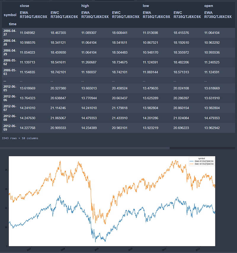
The first step is to take a look at the raw data from the ETFs EWA (Australia) and EWC (Canada):

Code output:

We can check if these ETFs are stationary by applying the Augmented Dickey-Fuller test, implemented in the statstools package.

Augmented Dickey Fuller results ('close', 'EWA R735QTJ8XC9X'):
stat=-1.950, p=0.309
Probably not Stationary
Augmented Dickey Fuller results ('close', 'EWC R735QTJ8XC9X'):
stat=-1.954, p=0.307
Probably not Stationary

As we expected, none of these series are stationary, however they seem to be highly correlated. Performing a linear regression between EWC and EWA, we find slope=1.312 and intercept=3.47.

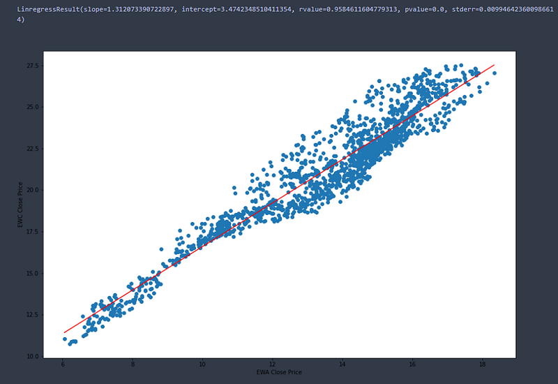
It means that, in general, considering the linear equation, we have the following relationship satisfied:

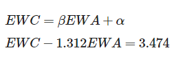
If we create an integrated portfolio EWC — 1.312EWA and plot it over time we obtain the graph from the next Figure, and we could also test it for stationarity.

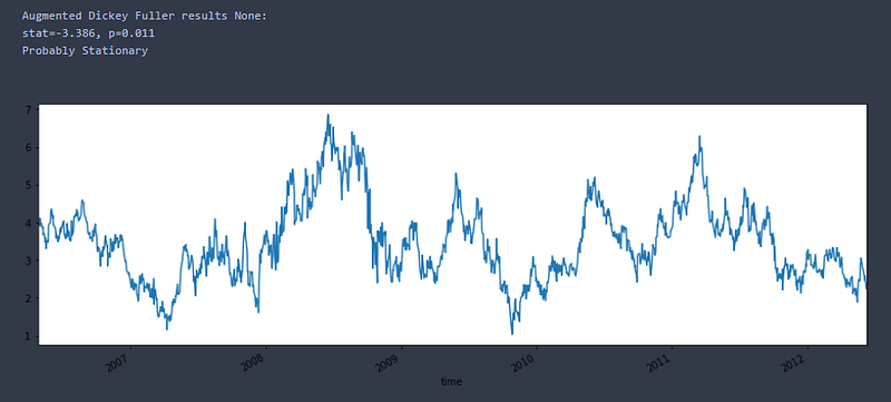
Note that this combined portfolio is now probably stationary, reverting to its mean (3.474) from time to time. This is the series that we should use for signaling entry and exit points, whenever the series move far from its mean.

Note: One important thing to keep in mind is that our portfolio has long and short positions at the same time. So, when we enter long (buy) we should buy EWC and short (sell) EWA and vice-versa.

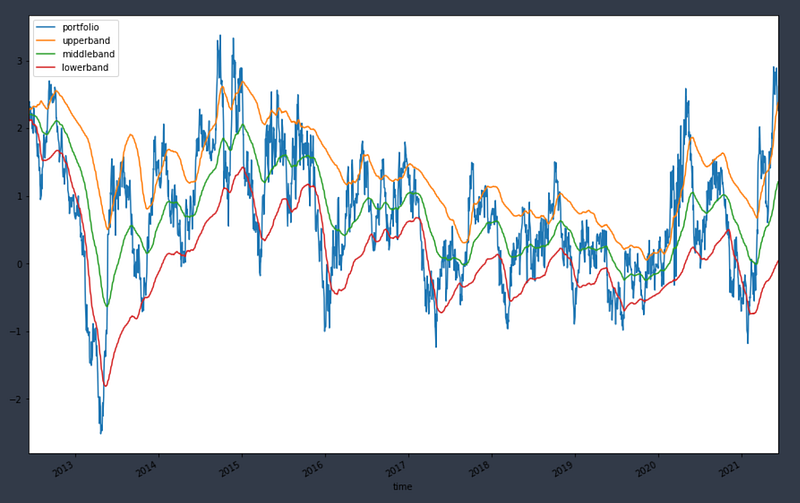
Defining Entry and Exit Signals

Once we have explained the underlying concept of the strategy, the next step is to define the entry and exit signals. We will apply the concept of Z-score, that is the number of standard deviations off the mean. To avoid incurring in look-ahead bias, we cannot backtest our strategy in the same time window we used to fit the data, so we will backtest it in a subsequent period (2012-now). The problem here is that we cannot use this same mean to trade the subsequent period because it may change, so what we do is to define a lookback window to create a dynamic moving average mean. We can do this using the Bollinger band indicator where the middle value is the mean (simple or exponential moving average) and the upper and lower bands are the mean +- a defined number of standard deviations (z-scores).

There is a big fall in the combined portfolio around 2013. That is probably due to a difference in the hedge ratio between the two assets in this period. This is a shortcoming of this simple strategy. In the future we will see a strategy that implements a dynamically assigned hedge ratio.

Implementing the Strategy

Now that we have all the theoretical pieces for our strategy, it is time to get into the algorithm code. It is not object of this tutorial to go deep into the Quantconnect engine, but I will try to write as many comments as possible directly into the code to make it easier to understand. So let’s do it.

Conclusion

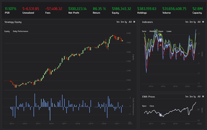
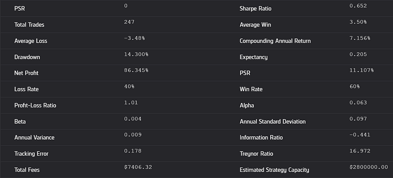
The results of this backtest from 2012 to 2021 can be seen in Figures 3 (chart) and 4 (report). We can see that the results are somewhat consistent but not exceptional as those achieved by Chan’s himself. Instead of an annualized return of 12.6% and a Sharpe ratio of 1.4, we achieved a more modest APR of 8% and 0.65 for Sharpe ratio, already considering the brokerage fees. We have to take into account also the differences in the time windows.

The backtest results as well as the code from the algorithm and the research notebook can be accessed in the following link:

My idea for the next posts is to continue implementing other algorithms in the Quantconnect platform to compare the results with those presented in the book. Two new versions of the mean reversion strategy, both with dynamicaly assigned hedge ratios and one with the Kalmann Filter (please refer to the post Understanding and Implementing Kalman Filter for Pairs Trading for more information) are on the way. So, if you liked the post and think it is helpful or have suggestions on how to improve it, please don’t hesitate to leave me a message. See you in the next story!

Update

Part 2 is already available:

Stay Connected

If you liked this article and want to continue reading/learning these and other stories without limits, consider becoming a Medium member. I’ll receive a portion of your membership fee if you use the following link, for no extra cost.

References

[1] Understanding and Implementing Kalman Filter for Pairs Trading | By Mauricio Cordeiro | Analytics Vidhya | Medium

[2] Chan, E., 2016. Algorithmic Trading: Winning Strategies and Their Rationale. Hoboken, N.J.: Wiley.