
Immensely Improving Every ‘Walmart Sales’ Forecasting Model
Simplicity is key.
“To better understand the marketplace, it is incumbent for organizations to look beyond their own four walls for data sources.”
Douglas Laney (VP, Gartner Research)
Intro
There have been several implementations of the popular Walmart Sales Forecast competition to predict their sales.

However, all of them seem to attempt to increase accuracy (reduce error) by focusing on mainly two things:
1) Feature engineering (getting the most out of your features)
2) Model/parameter optimization (choosing best model & best parameters)
Both of the above are very necessary indeed, but there is a third thing that adds value in a complementary way, and it’s wildly underused not only in this use case (which understandably was against the rules of the competition) but in most data science projects:
- Combining external information.
In this article, we’ll do a simple sales forecast model and then blend external variables (properly done).
The title of this article refers to improving all models, not because of doing something else, but by doing the same thing with more useful data.
So we’ll use the same model and we won’t do data wrangling or engineering at any point, so that we can tell apart only the benefit of adding useful features.
What we’ll do
- Step 1: Define and understand Target
- Step 2: Make a Simple Forecast Model
- Step 3: Add Financial Indicators and News
- Step 4: Test the Models
- Step 5: Measure Results
Step 1. Define and understand Target
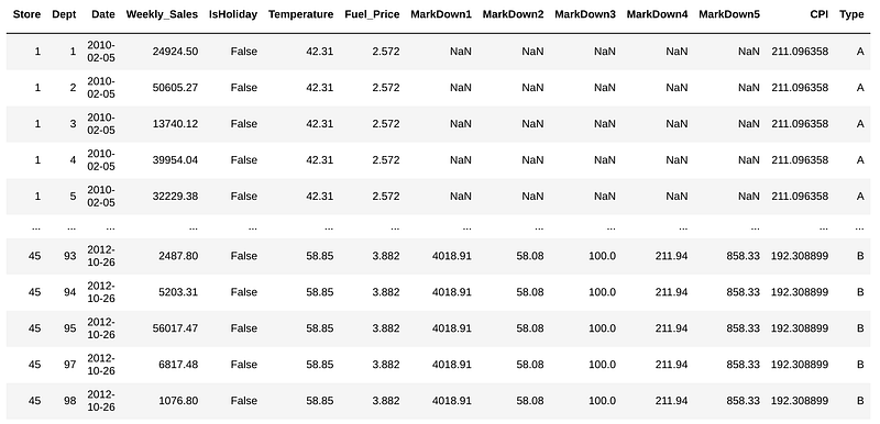
Walmart released data containing weekly sales for 99 departments (clothing, electronics, food…) in every physical store along with some other added features.
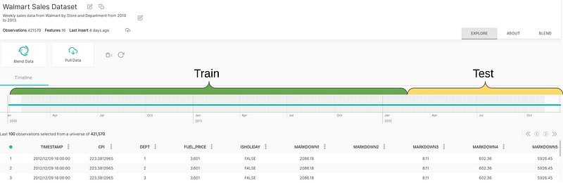
For this, we will create an ML model with ‘Weekly_Sales’ as target, and train with the first 70% observations and test on the posterior 30%.
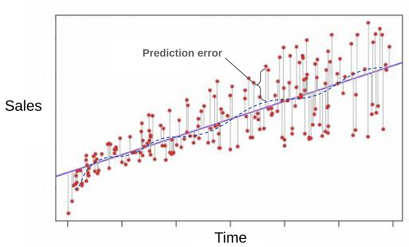
The objective is to minimize the Prediction error on future weekly sales.
We’ll add external variables that impact or have a relationship with sales such as dollar index, oil price and news about Walmart.
We won’t use model/parameter optimization nor feature engineering so we can distinguish the benefit from adding the external features.
Step 2. Make a Simple Forecast Model
First, you need to have Python 2 or 3 installed and the following libraries:
$ pip install pandas OpenBlender scikit-learnThen, open a Python script (preferably Jupyter notebook) and let’s import the needed libraries.
from sklearn.ensemble import RandomForestRegressor
import pandas as pd
import OpenBlender
import json
Now, let’s define the methodology and model to be used on all experiments.
First, the date range of the data is from Jan 2010 to Dec 2012. Let’s define the first 70% of the data used for training and the posterior 30% for testing (because we don’t want data leakage on our predictions).
Next, let’s define as our standard model a RandomForestRegressor with 50 estimators, which is a reasonably good option.
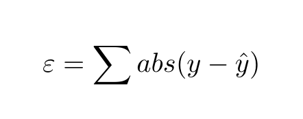
Finally, to keep things as simple as possible, let’s define the error as the absolute sum of errors.
Now, let’s put it in a Python class.
class StandardModel:

    model = RandomForestRegressor(n_estimators=50, criterion='mse')


    def train(self, df, target):
# Drop non numerics
df = df.dropna(axis=1).select_dtypes(['number']) # Create train/test sets
X = df.loc[:, df.columns != target].values
y = df.loc[:,[target]].values # We take the first bit of the data as test and the
# last as train because the data is ordered desc.
div = int(round(len(X) * 0.29)) X_train = X[div:]
y_train = y[div:] print('Train Shape:')
print(X_train.shape)
print(y_train.shape) #Random forest model specification
self.model = RandomForestRegressor(n_estimators=50) # Train on data
self.model.fit(X_train, y_train.ravel())
   def getMetrics(self, df, target):
        # Function to get the error sum from the trained model
# Drop non numerics
df = df.dropna(axis=1).select_dtypes(['number']) # Create train/test sets
X = df.loc[:, df.columns != target].values
y = df.loc[:,[target]].values div = int(round(len(X) * 0.29)) X_test = X[:div]
y_test = y[:div] print('Test Shape:')
print(X_test.shape)
print(y_test.shape)
# Predict on test
y_pred_random = self.model.predict(X_test) # Gather absolute error
error_sum = sum(abs(y_test.ravel() - y_pred_random)) return error_sumAbove we have an object with 3 elements:
- model (RandomForestRegressor)
- train: A function to train that model with a dataframe and a target
- getMetrics: A function to test with the trained model with the test data and retrieve the error
We will use this configuration for all of the experiments, although you can modify it as you want to test different models, parameters, configuration or whatever else. The value added will remain and could potentially improve.
Now, let’s get the Walmart data. You can get that csv here.
df_walmart = pd.read_csv('walmartData.csv')
print(df_walmart.shape)
df_walmart.head()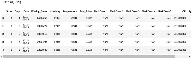
There are 421, 570 observations. As we said before, the observations are registers of weekly sales by store per department.
Let's plug the data into the model without tampering with it at all.
our_model = StandardModel()
our_model.train(df_walmart, 'Weekly_Sales')
total_error_sum = our_model.getMetrics(df_walmart, 'Weekly_Sales')
print("Error sum: " + str(total_error_sum))> Error sum: 967705992.5034052The sum of all errors for the complete model is $ 967,705,992.5 USD from all the predictions vs. the real sales.
This doesn’t mean much by itself, the only reference is that the sum of all sales in that period is $ 6,737,218,987.11 USD.
Since there is a whole lot of data, we will only focus on Store #1 for this tutorial, but the methodology is absolutely replicable for all stores.
Let’s take a look at the error generated by Store 1 alone.
# Select store 1
df_walmart_st1 = df_walmart[df_walmart['Store'] == 1]
error_sum_st1 = our_model.getMetrics(df_walmart_st1, 'Weekly_Sales')
print("Error sum error_sum_st1: " + str(error_sum_st1))# > Error sum error_sum_st1: 24009404.060399983So, Store 1 is responsible for the $24,009,404.06 USD error and this will be our threshold for comparison.
Now let’s break down the error by department to have more visibility later.
error_summary = []for i in range(1,100):
try:
df_dept = df_walmart_st1[df_walmart_st1['Dept'] == i]
error_sum = our_model.getMetrics(df_dept, 'Weekly_Sales')
print("Error dept : " + str(i) + ' is: ' + str(error_sum))
error_summary.append({'dept' : i, 'error_sum_normal_model' : error_sum})
except:
error_sum = 0
print('No obs for Dept: ' + str(i))error_summary_df = pd.DataFrame(error_summary)
error_summary_df.head()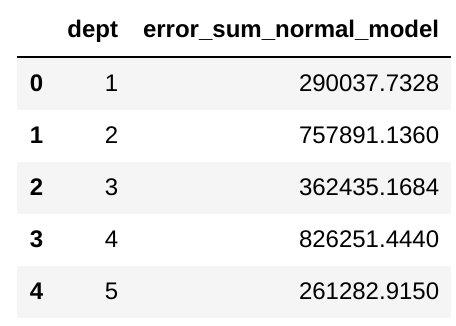
Now we have a dataframe with the errors corresponding to each department on Store 1 with our threshold model.
Let’s improve these numbers.
Step 3. Add Financial Indicators and News
Let’s select department 1 to make a simple example.
df_st1dept1 = df_walmart_st1[df_walmart_st1['Dept'] == 1]Now, lets prep the timestamp variable.
# First we need to add the UNIX timestamp which is the number
# of seconds since 1970 on UTC, it is a very convenient
# format because it is the same in every time zone in the world!df_st1dept1['timestamp'] = OpenBlender.dateToUnix(df_st1dept1['Date'],
date_format = '%Y-%m-%d',
timezone = 'GMT')df_st1dept1 = df_st1dept1.sort_values('timestamp').reset_index(drop = True)Now, let’s search for intersected (time overlapped) datasets about ‘business’ or ‘walmart’ in OpenBlender .
Note: To get a token you need have to create an account on openblender.io (free), you’ll find it in the ‘Account’ tab on your profile icon.


token = 'YOUR_TOKEN_HERE'print('From : ' + OpenBlender.unixToDate(min(df_st1dept1.timestamp)))print('Until: ' + OpenBlender.unixToDate(max(df_st1dept1.timestamp)))# Now, let's search on OpenBlender
search_keyword = 'business walmart'# We need to pass our timestamp column and
# search keywords as parameters.
OpenBlender.searchTimeBlends(token,
df_st1dept1.timestamp,
search_keyword)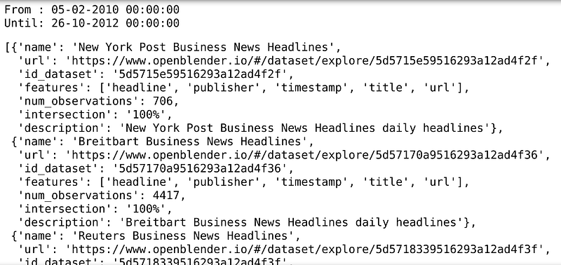
The search found several datasets. We can see name, description, url, features, and most importantly, time interesction with ours so we can blend them to our dataset.
Let’s start by blending this walmart tweets dataset and look for promos.
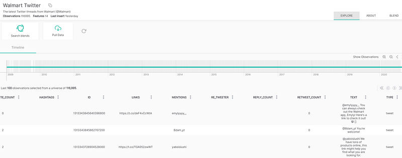
- Note: I picked this one because it makes sense, but you can search for hundreds of other ones.
We can blend new columns to our dataset by searching terms on texts or news aggregated by time. For instance, we could create a ‘promo’ feature with the number of mentions which will match our self made ngrams:
text_filter = {'name' : 'promo',
               'match_ngrams': ['promo', 'dicount', 'cut', 'markdown','deduction']}
# blend_source needs the id_dataset and the name of the feature.blend_source = {
'id_dataset':'5e1deeda9516290a00c5f8f6',
'feature' : 'text',
'filter_text' : text_filter
}df_blend = OpenBlender.timeBlend( token = token,
anchor_ts = df_st1dept1.timestamp,
blend_source = blend_source,
blend_type = 'agg_in_intervals',
interval_size = 60 * 60 * 24 * 7,
direction = 'time_prior',
interval_output = 'list')df_anchor = pd.concat([df_st1dept1, df_blend.loc[:, df_blend.columns != 'timestamp']], axis = 1)The parameters for the timeBlend function (you can find the documentation here):
- anchor_ts: We only need to send our timestamp column so that it can be used as an anchor to blend the external data.
- blend_source: The information about the feature we want.
- blend_type: ‘agg_in_intervals’ because we want 1 week interval aggregation to each of our observations.
- inverval_size: The size of the interval in seconds (24 * 7 hours in this case).
- direction: ‘time_prior’ because we want the interval to gather observations from the prior 7 days and not forward to avoid data leakage.
We now have our original dataset but with 2 new columns, the ‘COUNT’ of our ‘promo’ feature and a list of the actual texts in case one wants to iterate through each one.
df_anchor.tail()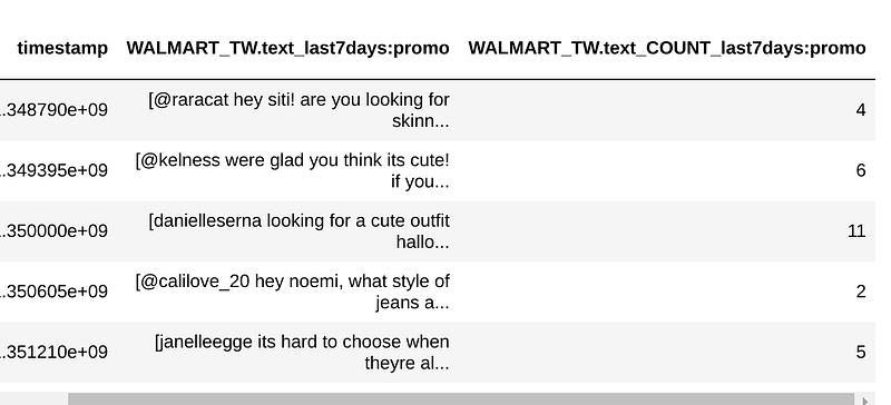
So now we have a numerical feature about how many times our ngrams were mentioned. We could probably do better ngrams if we knew which store or department corresponds to ‘1’ (Walmart didn’t share that).
Let’s apply the Standard Model and compare the error vs. the original.
our_model.train(df_anchor, 'Weekly_Sales')
error_sum = our_model.getMetrics(df_anchor, 'Weekly_Sales')
error_sum
#> 253875.30The current model had a $253, 975 error while the previous one had $290,037. That’s a 12% improvement.
But this doesn’t prove much, it could be that the RandomForest got lucky. After all, the original model trained with over 299K observations. The current one only training with 102!!
We can also blend numerical features. Let’s try blending Dollar index, Oil price, and Monthly Consumer Sentiment
# OIL
blend_source = {
                'id_dataset':'5e91045a9516297827b8f5b1',
                'feature' : 'price'
            }
df_blend = OpenBlender.timeBlend( token = token,
anchor_ts = df_anchor.timestamp,
blend_source = blend_source,
blend_type = 'agg_in_intervals',
interval_size = 60 * 60 * 24 * 7,
direction = 'time_prior',
interval_output = 'avg',
missing_values = 'impute')df_anchor = pd.concat([df_anchor, df_blend.loc[:, df_blend.columns != 'timestamp']], axis = 1)# DOLLAR INDEXblend_source = {
'id_dataset':'5e91029d9516297827b8f08c',
'feature' : 'price'
}df_blend = OpenBlender.timeBlend( token = token,
anchor_ts = df_anchor.timestamp,
blend_source = blend_source,
blend_type = 'agg_in_intervals',
interval_size = 60 * 60 * 24 * 7,
direction = 'time_prior',
interval_output = 'avg',
missing_values = 'impute')df_anchor = pd.concat([df_anchor, df_blend.loc[:, df_blend.columns != 'timestamp']], axis = 1)# CONSUMER SENTIMENTblend_source = {
'id_dataset':'5e979cf195162963e9c9853f',
'feature' : 'umcsent'
}df_blend = OpenBlender.timeBlend( token = token,
anchor_ts = df_anchor.timestamp,
blend_source = blend_source,
blend_type = 'agg_in_intervals',
interval_size = 60 * 60 * 24 * 7,
direction = 'time_prior',
interval_output = 'avg',
missing_values = 'impute')df_anchor = pd.concat([df_anchor, df_blend.loc[:, df_blend.columns != 'timestamp']], axis = 1)df_anchor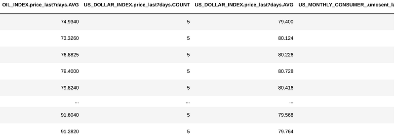
Now we have 6 more features, the average of oil index, dollar index and consumer sentiment on the 7 day intervals and the count of each (which for this case is irrelevant).
Let’s run that model again.
our_model.train(df_anchor, 'Weekly_Sales')
error_sum = our_model.getMetrics(df_anchor, 'Weekly_Sales')
error_sum>223831.9414Now, we’re down to a $223,831 error. That’s a 24.1% improvement with repect to the original $290,037 !!
So let’s now try it with every department separately to measure how consistent the benefit is.
Step 4. Test in All Departments
To get a glimpse, we’re gonna experiment with the first 10 Departments first and compare the benefit of adding each additional source.
# Function to filter features from other sourcesdef excludeColsWithPrefix(df, prefixes):
cols = df.columns
for prefix in prefixes:
cols = [col for col in cols if prefix not in col]
return df[cols]error_sum_enhanced = []action = 'API_getObservationsFromDataset'# Loop through the first 10 Departments and test them.for dept in range(1, 10):
print('---')
print('Starting department ' + str(dept))
# Get it into a dataframe
df_dept = df_walmart_st1[df_walmart_st1['Dept'] == dept]
# Unix Timestamp
df_dept['timestamp'] = OpenBlender.dateToUnix(df_dept['Date'],
date_format = '%Y-%m-%d',
timezone = 'GMT')# Function to filter features from other sourcesdef excludeColsWithPrefix(df, prefixes):
cols = df.columns
for prefix in prefixes:
cols = [col for col in cols if prefix not in col]
return df[cols]error_sum_enhanced = []# Loop through the first 10 Departments and test them.for dept in range(1, 10):
print('---')
print('Starting department ' + str(dept))
# Get it into a dataframe
df_dept = df_walmart_st1[df_walmart_st1['Dept'] == dept]
# Unix Timestamp
df_dept['timestamp'] = OpenBlender.dateToUnix(df_dept['Date'],
date_format = '%Y-%m-%d',
timezone = 'GMT')df_dept = df_dept.sort_values('timestamp').reset_index(drop = True)
# "PROMO" FEATURE OF MENTIONS ON WALMART
text_filter = {'name' : 'promo',
'match_ngrams': ['promo', 'dicount', 'cut', 'markdown','deduction']}
blend_source = {
'id_dataset':'5e1deeda9516290a00c5f8f6',
'feature' : 'text',
'filter_text' : text_filter
}df_blend = OpenBlender.timeBlend( token = token,
anchor_ts = df_st1dept1.timestamp,
blend_source = blend_source,
blend_type = 'agg_in_intervals',
interval_size = 60 * 60 * 24 * 7,
direction = 'time_prior',
interval_output = 'list')df_anchor = pd.concat([df_st1dept1, df_blend.loc[:, df_blend.columns != 'timestamp']], axis = 1)
# OIL
blend_source = {
'id_dataset':'5e91045a9516297827b8f5b1',
'feature' : 'price'
}df_blend = OpenBlender.timeBlend( token = token,
anchor_ts = df_anchor.timestamp,
blend_source = blend_source,
blend_type = 'agg_in_intervals',
interval_size = 60 * 60 * 24 * 7,
direction = 'time_prior',
interval_output = 'avg',
missing_values = 'impute')df_anchor = pd.concat([df_anchor, df_blend.loc[:, df_blend.columns != 'timestamp']], axis = 1)# DOLLAR INDEXblend_source = {
'id_dataset':'5e91029d9516297827b8f08c',
'feature' : 'price'
}df_blend = OpenBlender.timeBlend( token = token,
anchor_ts = df_anchor.timestamp,
blend_source = blend_source,
blend_type = 'agg_in_intervals',
interval_size = 60 * 60 * 24 * 7,
direction = 'time_prior',
interval_output = 'avg',
missing_values = 'impute')df_anchor = pd.concat([df_anchor, df_blend.loc[:, df_blend.columns != 'timestamp']], axis = 1)# CONSUMER SENTIMENTblend_source = {
'id_dataset':'5e979cf195162963e9c9853f',
'feature' : 'umcsent'
}df_blend = OpenBlender.timeBlend( token = token,
anchor_ts = df_anchor.timestamp,
blend_source = blend_source,
blend_type = 'agg_in_intervals',
interval_size = 60 * 60 * 24 * 7,
direction = 'time_prior',
interval_output = 'avg',
missing_values = 'impute')df_anchor = pd.concat([df_anchor, df_blend.loc[:, df_blend.columns != 'timestamp']], axis = 1)
try:
error_sum = {}
# Gather errors from every source by itself# Dollar Index
df_selection = excludeColsWithPrefix(df_anchor, ['WALMART_TW', 'US_MONTHLY_CONSUMER', 'OIL_INDEX'])
our_model.train(df_selection, 'weekly_sales')
error_sum['1_features'] = our_model.getMetrics(df_selection, 'weekly_sales')
# Walmart News
df_selection = excludeColsWithPrefix(df_anchor, [ 'US_MONTHLY_CONSUMER', 'OIL_INDEX'])
our_model.train(df_selection, 'weekly_sales')
error_sum['2_feature'] = our_model.getMetrics(df_selection, 'weekly_sales')
# Oil Index
df_selection = excludeColsWithPrefix(df_anchor,['US_MONTHLY_CONSUMER'])
our_model.train(df_selection, 'weekly_sales')
error_sum['3_features'] = our_model.getMetrics(df_selection, 'weekly_sales')
# Consumer Sentiment (All features)
df_selection = df
our_model.train(df_selection, 'weekly_sales')
error_sum['4_features'] = our_model.getMetrics(df_selection, 'weekly_sales')
except:
print(traceback.format_exc())
print("No observations found for department: " + str(dept))
error_sum = 0
error_sum_enhanced.append(error_sum)Let’s get the results into a DataFrame and visualize.
separated_results = pd.DataFrame(error_sum_enhanced)
separated_results['original_error'] = error_summary_df[0:10]['error_sum_normal_model']
separated_results = separated_results[['original_error', '1_feature', '2_features', '3_features', '4_features']]
separated_resultsseparated_results.transpose().plot(kind='line')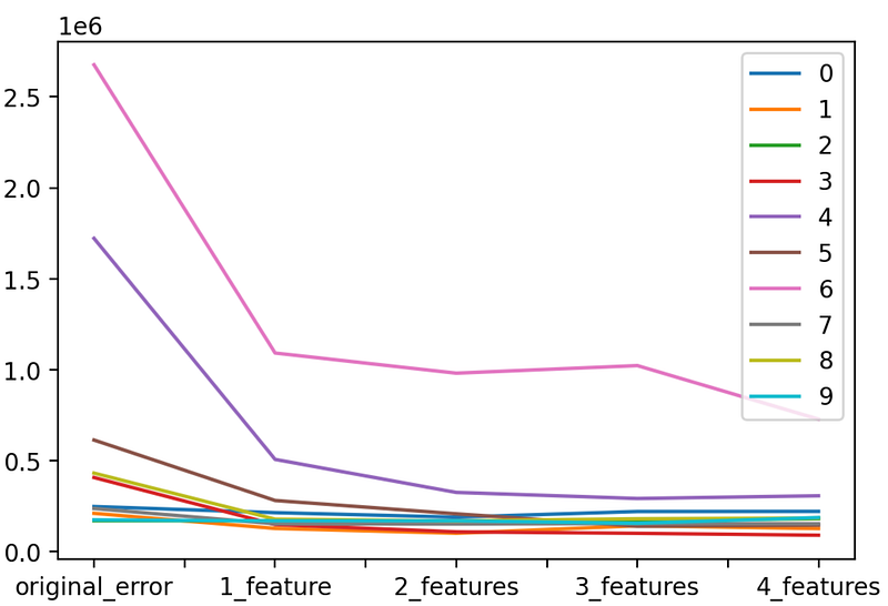
Departments 4 and 6 are on a higher order than the rest Let’s remove them to take a closer look at the rest.
separated_results.drop([6, 4]).transpose().plot(kind=’line’)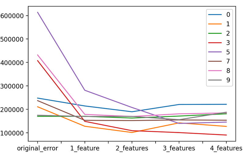
We can see that almost on all departments the error lowered as we added new features. We can also see that the Oil Index (third feature) was not only not helpful but even harmful for some departments.
I excluded the Oil Index and ran the algorithm with the 3 features on all the departments (which you can do by iterating all the error_summary_df and not just the first 10).
Let’s see the results.
Step 5. Measure Results
These are the results of the ‘3 feature’ blend and the improvement percentage on all departments:
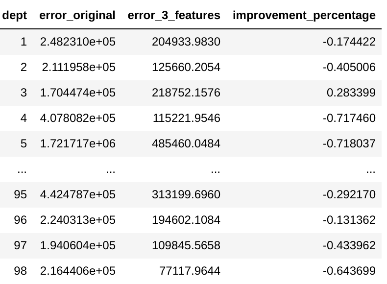
Not only did the added features improve the error on over 88% of the Departments, but some improvements were significant.
This is the histogram for the improvement percentage.
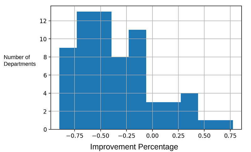
The original error (calculated at the beginning of the article) was $24,009,404.06 USD, and the final error is $9,596,215.21 USD meaning it was reduced by over 60%
And this is just one store.
Thank you for reading.


