Imbalanced Multi-Class Classification: Balanced Weights May Not Improve Your Model Performance

Compare the random forest model and logistic regression model with and without balanced weights on imbalanced multi-class classification

The balanced weight is a widely used method for imbalanced classification models. It penalizes the wrong predictions about the minority classes by giving more weight to the loss function.

In this tutorial, we will talk about how to use balanced weight for the imbalanced multi-class classification. We will cover the following:

• What is the algorithm behind the balanced class weights for multi-classes?
• How to use class weights on random forest and logistic regression for multi-class classification?
• How to interpret the model performance metrics of a multi-class classification model?
• How to decide whether to use the balanced weights for an imbalanced multi-class classification model?

If you are interested in the balanced weight for a binary classification model, please check out my previous tutorial Balanced Weights For Imbalanced Classification.

Resources for this post:

• Video tutorial for this post on YouTube
• Click here for the Colab notebook
• More video tutorials on imbalanced modeling and anomaly detection
• More blog posts on imbalanced modeling and anomaly detection

Let’s get started!

Step 1: Import Libraries

The first step is to import libraries.

• make_classification from sklearn is for creating the modeling dataset.
• pandas and numpy are for data processing
• Counter counts the number of records.
• matplotlib and seaborn are for visualization.
• train_test_split is for creating the training and the validation datasets.
• RandomForestClassifier and LogisticRegression are for modeling.
• class_weight is for adjusting weights.
• classification_report is for model performance evaluation.

# Synthetic dataset
from sklearn.datasets import make_classification

# Data processing
import pandas as pd
import numpy as np
from collections import Counter

# Data visualization
import matplotlib.pyplot as plt
import seaborn as sns

# Model and performance
from sklearn.model_selection import train_test_split
from sklearn.ensemble import RandomForestClassifier
from sklearn.linear_model import LogisticRegression
from sklearn.utils import class_weight
from sklearn.metrics import classification_report

Step 2: Create Imbalanced Dataset

In step 2, we will create a synthetic multi-class imbalanced dataset for the classification model using make_classification from the sklearn library.

• n_samples=100000 indicates that 100000 samples will be generated.
• n_features is the number of predictors.
• n_informative is the number of informative predictors.
• n_redundant is the number of redundant predictors, which are the linear combinations of the informative predictors.
• n_repeated is the number of duplicated predictors, which are randomly selected from the informative and the redundant features.
• n_classes=3 means that there are 3 classes in the dependent variable.
• n_clusters_per_class=1 indicates that there are no clusters within each class.
• weights specifies the percentage of samples in each class.
• class_sep indicates how separable the classes are. Larger values spread out the classes and make the classification predictions easier.
• random_state makes the synthetic dataset reproducible.

The output of the synthetic dataset is in numpy array format. We converted it into the pandas dataframe format.

# Create an imbalanced dataset
X, y = make_classification(n_samples=100000, n_features=2, n_informative=2,
                           n_redundant=0, n_repeated=0, n_classes=3,
                           n_clusters_per_class=1,
                           weights=[0.97, 0.02, 0.01],
                           class_sep=0.8, random_state=0)

# Convert the data from numpy array to a pandas dataframe
df = pd.DataFrame({'feature1': X[:, 0], 'feature2': X[:, 1], 'target': y})

# Check the target distribution
df['target'].value_counts(normalize = True)

Output:

0    0.96321
1    0.02347
2    0.01332
Name: target, dtype: float64

The distribution of the target variable shows that we have about 96% of samples for class 0, 2% of the samples for class 1, and 1% of the samples for class 2.

# Set figure size
plt.figure(figsize=(12, 8))

# Count plot
sns.countplot(x='target', data=df, order=df['target'].value_counts().index)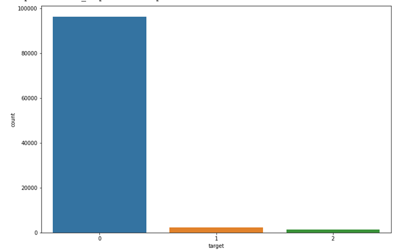

The scatter plot shows the distribution of the data points.

# Set figure size
plt.figure(figsize=(12, 8))

# Scatter plot
sns.scatterplot(x = 'feature1', y = 'feature2', hue = 'target', data = df)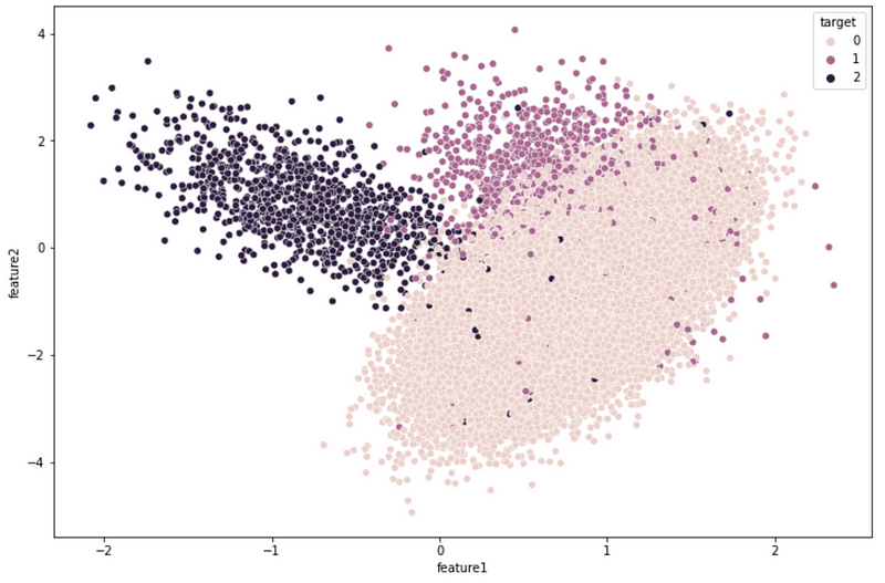

Step 3: Train Test Split

In step 3, we will split the dataset into 80% training and 20% validation datasets. random_state ensures that we have the same train test split every time.

# Train test split
X_train, X_test, y_train, y_test = train_test_split(X, y, test_size=0.2, random_state=42)

# Check the number of records
print('The number of records in the training dataset is', X_train.shape[0])
print('The number of records in the test dataset is', X_test.shape[0])
print(f"The training dataset has {sorted(Counter(y_train).items())[0][1]} records for the class 0, {sorted(Counter(y_train).items())[1][1]} records for class 1 and {sorted(Counter(y_train).items())[2][1]} records for class 2.")

The train test split gives us 80,000 records for the training dataset and 20,000 for the validation dataset. The training dataset has 77,058 records for class 0, 1,869 records for class 1, and 1,073 records for class 2.

Step 4: Baseline Multi-class Random Forest Classification

In step 4, we will build a baseline multi-class classification model with random forest using the imbalanced dataset.

• RandomForestClassifier is the method for the random forest classification model. random_state=0 set the seed for the random splits to make them reproducible. n_jobs=-1 enables parallel processing.
• .fit takes in X_train and y_train for model fitting.
• .predict takes in X_test for testing dataset prediction. It produces the predicted labels for all the testing dataset records.

# Train the random forest model using the imbalanced dataset
baseline_rf = RandomForestClassifier(random_state=0, n_jobs=-1).fit(X_train, y_train)

# Baseline model prediction
y_test_pred_baseline = baseline_rf.predict(X_test)

# Take a look at the prediction
y_test_pred_baseline[:5]

Output:

array([0, 0, 0, 0, 0])

Step 5: Multi-class Metrics Interpretation

In step 5, we will use the classification_report to evaluate the baseline multi-class classification random forest model performance.

# Evaluation metrics
print(classification_report(y_test,y_test_pred_baseline))

Output:

              precision    recall  f1-score   support

           0       0.98      1.00      0.99     19263
           1       0.70      0.25      0.36       478
           2       0.97      0.67      0.79       259

    accuracy                           0.98     20000
   macro avg       0.88      0.64      0.72     20000
weighted avg       0.97      0.98      0.97     20000

The classification_report compares the actual and predicted labels for the testing dataset. The output has two sections, the top section for the metrics by class and the bottom section for the overall metrics.

• precision is the percentage of correct predictions for the predicted class. For example, the precision value of 0.98 for class 0 indicates that 98% of the predicted class 0 are actual class 0.
• recall is the percentage of samples captured by the model for the class. For example, the recall value of 0.25 for class 1 indicates that 25% of the samples in class 1 are captured by the model.
• f1-score is the harmonic value of precision and recall. It is 2*precision*recall/(precision+recall). For example, the f1-score for class 2 is calculated using 2*0.97*0.67/(0.97+0.67)=0.79.
• support for the top section has the count of samples for each class.

The bottom section of classification_report has the overall metrics across all the classes.

• accuracy is the percentage of correct predictions across all classes.
• macro avg is the unweighted mean of a metric across all the classes. For example, macro avg for precision is calculated by (0.98+0.70+0.97)/3=0.88. It's a good metric to look at for a balanced dataset because it gives equal weights to each class.
• weighted avg is the weighted mean of a metric across all the classes. For example, weighted avg for recall is calculated by 1*0.96321+0.25*0.02347+0.67*0.01332=0.978. It's a good metric to look at for an imbalanced dataset because it takes the weighted average based on class proportion.
• support for the bottom section has the total number of samples for the testing dataset.

Step 6: Algorithm Behind Balanced Weights

In step 6, we will talk about the algorithm behind the balanced weights.

The weights are calculated using the inverse proportion of the class frequencies. The rationale behind it is that the model penalizes more for the wrong predictions on low-frequency classes.

np.unique(y_train, return_counts=True) gives us the unique label values of all the classes and their corresponding number of records.

# Frequencies by class labels
unique, counts = np.unique(y_train, return_counts=True)

# Print the frequencies
print(np.asarray((unique, counts)).T)

Output:

[[    0 77058]
 [    1  1869]
 [    2  1073]]

The proportion of a class is the number of records of the class divided by the total number of records in the training dataset, and the inverse proportion of a class is 1 over the proportion of a class.

# Calculate weights manually
print(f'The weights for class 0 is {1/(77058/80000):.3f}')
print(f'The weights for class 1 is {1/(1869/80000):.3f}')
print(f'The weights for class 2 is {1/(1073/80000):.3f}')

We can see that the weight for class 0 is 1.038, the weight for class 1 is 42.804, and the weight for class 2 is 74.557.

The weights for class 0 is 1.038
The weights for class 1 is 42.804
The weights for class 2 is 74.557

sklearn has a built-in utility function class_weight.compute_class_weight for calculating the class weights.

• class_weight='balanced' implements the inverse proportion of classes as the weights for the loss function.
• classes takes in the unique values of the classes.
• y=y_train means that the name for the dependent variable of the training dataset is y_train.

# Calculate weights using sklearn
sklearn_weights = class_weight.compute_class_weight(class_weight='balanced', 
                                                    classes=np.unique(y_train), 
                                                    y=y_train)

# Take a look at the values
sklearn_weights

Output:

array([ 0.34605968, 14.26787944, 24.85243865])

The outputs from compute_class_weight are 0.34, 14.27, and 24.85. If we multiply each weight by 3, the results are the same as our manual calculation. This is because the formula for compute_class_weight is n_samples / (n_classes * np.bincount(y)). There are 3 classes, so the values are 3 times the inverse proportion of each class.

# Compare the values
print(f'The weights for class 0 is {sklearn_weights[0]*3:.3f}')
print(f'The weights for class 1 is {sklearn_weights[1]*3:.3f}')
print(f'The weights for class 2 is {sklearn_weights[2]*3:.3f}')

Output:

The weights for class 0 is 1.038
The weights for class 1 is 42.804
The weights for class 2 is 74.557

Step 7: Balanced Weights For Multi-class Random Forest Model

In step 7, we will train a random forest multi-class model with the balanced weight.

class_weight is a parameter of RandomForestClassifier.

• The default value for class_weight is None, meaning that all classes have the same weight of 1.
• class_weight='balanced' uses the values of y_train to automatically calculate the inverse proportion of class frequencies with the formula n_samples / (n_classes * np.bincount(y)).
• class_weight='balanced_subsample' has the same calculation as class_weight='balanced' except that weights are computed based on the bootstrap samples for each tree.
• class_weight can also take a dictionary or a list of dictionaries for customized weights.

# Train the random forest model using the imbalanced dataset
balanced_rf = RandomForestClassifier(class_weight='balanced', random_state=0, n_jobs=-1).fit(X_train, y_train)

# Baseline model prediction
y_test_pred_balanced = balanced_rf.predict(X_test)

# Evaluation metrics
print(classification_report(y_test, y_test_pred_balanced))

We can see that the multi-class random forest model with class_weight='balanced' has very similar performance as the baseline random forest model across all the metrics, indicating that the balanced weight does not improve the performance of the random forest model on the imbalanced multi-class dataset.

              precision    recall  f1-score   support

           0       0.98      1.00      0.99     19263
           1       0.73      0.23      0.35       478
           2       0.98      0.67      0.79       259

    accuracy                           0.98     20000
   macro avg       0.90      0.63      0.71     20000
weighted avg       0.97      0.98      0.97     20000

Next, let’s try class_weight='balanced_subsample' and calculate the weights based on the samples for each tree.

# Train the random forest model using the imbalanced dataset
balanced_subsample_rf = RandomForestClassifier(class_weight='balanced_subsample', random_state=0, n_jobs=-1).fit(X_train, y_train)

# Baseline model prediction
y_test_pred_balanced_subsample = balanced_rf.predict(X_test)

# Evaluation metrics
print(classification_report(y_test, y_test_pred_balanced_subsample))

We got the same performance metric values as the random forest model with the class_weight='balanced' option, indicating that the balanced weights do not have a positive impact on the random forest model on this dataset.

              precision    recall  f1-score   support

           0       0.98      1.00      0.99     19263
           1       0.73      0.23      0.35       478
           2       0.98      0.67      0.79       259

    accuracy                           0.98     20000
   macro avg       0.90      0.63      0.71     20000
weighted avg       0.97      0.98      0.97     20000

Is this the case just for the random forest model? Let’s try the balanced weights on logistic regression and see if it makes a difference.

Step 8: Baseline Multi-class Logistic Regression

In step 8, we will build a baseline multi-class classification model with logistic regression using the imbalanced dataset.

# Train the random forest model using the imbalanced dataset
baseline_lr = LogisticRegression(random_state=0, n_jobs=-1).fit(X_train, y_train)

# Baseline model prediction
y_test_pred_baseline = baseline_lr.predict(X_test)

# Evaluation metrics
print(classification_report(y_test, y_test_pred_baseline))

Compared with the classification_report from the random forest model, the logistic regression baseline model has similar performance on class 0 and class 2.

              precision    recall  f1-score   support

           0       0.97      1.00      0.99     19263
           1       0.97      0.13      0.24       478
           2       0.99      0.64      0.78       259

    accuracy                           0.97     20000
   macro avg       0.98      0.59      0.67     20000
weighted avg       0.97      0.97      0.97     20000

For class 1, logistic regression has a precision of 0.97, higher than the random forest baseline model precision of 0.70. Logistic regression has a recall of 0.13, lower than the random forest baseline model recall of 0.25. Logistic regression has an f1-score of 0.24, lower than the random forest baseline model recall of 0.36.

We can see that if the goal is to get high precision, the baseline logistic regression has good results across all the classes. But if the goal is to get high recall values, the baseline logistic regression has a poor performance.

Step 9: Balanced Weights For Multi-class Logistic Regression Model

In step 9, we will train a random forest multi-class model with the balance weight.

class_weight is a parameter of LogisticRegression.

• The default value for class_weight is None, meaning that all classes have the same weight of 1.
• class_weight='balanced' uses the values of y_train to automatically calculate the inverse proportion of class frequencies with the formula n_samples / (n_classes * np.bincount(y)).
• class_weight can also take a dictionary for customized weights.

# Train the random forest model using the imbalanced dataset
balanced_lr = LogisticRegression(class_weight='balanced', random_state=0, n_jobs=-1).fit(X_train, y_train)

# Baseline model prediction
y_test_pred_baseline = balanced_lr.predict(X_test)

# Evaluation metrics
print(classification_report(y_test, y_test_pred_baseline))

What a big difference the balanced weights made on the logistic regression! From the classification_report output, we can see that the recall values for all the classes are similar. The recall for class 1 increased from 0.13 to 0.73 and the recall for class 2 increased from 0.64 to 0.72. However, the precision for class 1 and class 2 decreased.

              precision    recall  f1-score   support

           0       0.99      0.72      0.84     19263
           1       0.07      0.73      0.13       478
           2       0.19      0.72      0.30       259

    accuracy                           0.72     20000
   macro avg       0.42      0.72      0.42     20000
weighted avg       0.96      0.72      0.81     20000

Therefore, if the goal of the project is to achieve higher recall values, class_weight='balanced' should be used with the logistic regression model. If the goal of the project is to maximize precision, the default class_weight=None should be used with the logistic regression model.

Summary

From the comparisons between random forest and logistic regression and the comparisons between with and without the balanced weights for the loss function, we can see that

• The balanced weight parameter may or may not improve the model performance, so having a baseline model before applying class_weight='balanced' on an imbalanced dataset is important.
• Depending on the specific goal of the project, using a baseline model can perform a lot better than using a model with class_weight='balanced'. For example, in the example above, we saw logistic regression baseline model has over 90% precision for all three classes, but under 20% precision for the two minority classes after applying class_weight='balanced'.
• Different machine learning algorithms can have quite different results for imbalanced multi-class classification. Therefore, it’s important to compare different algorithms and pick the model that aligns best with the goal of the project.

More tutorials are available on GrabNGoInfo YouTube Channel, GrabNGoInfo.com, and LinkedIn.

Recommended Tutorials

• GrabNGoInfo Machine Learning Tutorials Inventory
• Balanced Weights For Imbalanced Classification
• Hierarchical Topic Model for Airbnb Reviews
• 3 Ways for Multiple Time Series Forecasting Using Prophet in Python
• Time Series Anomaly Detection Using Prophet in Python
• Time Series Causal Impact Analysis in Python
• Hyperparameter Tuning For XGBoost
• Four Oversampling And Under-Sampling Methods For Imbalanced Classification Using Python

References

• sklearn documentation on make_classification
• sklearn documentation on compute_class_weight
• Random Forest Classifier in sklearn
• Logistic Regression in sklearn