Summary

The website content discusses the impact of hyperparameter tuning and data ratios on the performance of linear regression models in classifying imbalanced datasets.

Abstract

The article explores the effects of varying data ratios and the hyperparameter 'C' in linear regression models to address imbalanced datasets. Experiments were conducted using four different data ratios of blue to red points, ranging from highly imbalanced to nearly balanced, and three distinct values of 'C' (0.001, 1, 100). The results indicate that both the data ratio and the value of 'C' significantly influence the decision line's placement and the model's classification accuracy. A higher 'C' value generally leads to a better fit, but beyond a certain threshold, it may cause overfitting. The findings suggest that careful tuning of the model and the hyperparameter 'C' is crucial for achieving an optimal classification model.

Opinions

The author believes that the hyperparameter 'C' has a substantial impact on the linear regression model's performance, as evidenced by the shifting position of the decision line in response to changes in 'C'.
The article posits that increasing the data ratio towards a more balanced dataset improves the model's ability to classify data points accurately.
It is the author's opinion that while a higher 'C' value can enhance the model's fit, there is a point at which further increases will result in overfitting, which should be avoided.
The author emphasizes the importance of both data ratio and hyperparameter tuning in developing an effective linear regression model for imbalanced datasets.
The conclusion of the article encourages readers to train and tune their models wisely, suggesting that there is a skillful approach to model development that can lead to better outcomes.

Imbalanced data and Linear regression

Linear Regression (LR) is used for finding linear relationship between target and one or more predictors. The core idea is to obtain a line that best fits the data. The best fit line is the one for which total prediction error(all data points) are as small as possible. Error is the distance between the point to the regression line. In this blog we will cover various set hyper parameter of linear regression model and performing prediction models.

Linear regression assumes that the relationship between the features and the target vector is approximately linear. That is, the effect (also called coefficient, weight, or parameter) of the features on the target vector is constant. In our solution, for the sake of explanation we have trained our model using only two features.

In our experiment, we took 4 set of data in different ratios that are [(100:2),(100:20),(100:40),(100:80)] and 3 set of hyper parameter ‘C’ that are [0.001, 1, 100]. We are going to see the results of all these 12 combinations and will analyze them one by one.

Set 1 :- Data ratio = (100:2) ->(blue : red)

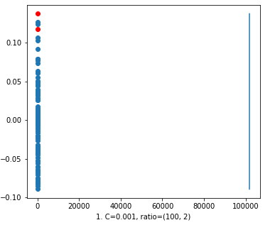
First we took the value of ‘C’=0.001. In the resultant figure 1 the decision line is at 100k on X-axis and it is far from classification because the data on the left most side but the decision line on the right most side, even though we have 2 red points are with 100 blue points.

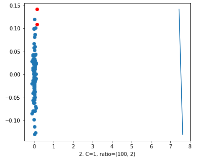
Now, coming to the 2nd figure, we increased the value of ‘C’ = 1. Many of you will think that there isn’t any difference between figure 1 and figure 2. But, look again at the x-axis. In figure 1 the data points were on 0 and the decision line was on 100k. In figure 2, the data is around 0 and x-axis and the decision line has come so close to 8 on x-axis. So, we can say that there is a great impact of ‘C’ on data set.

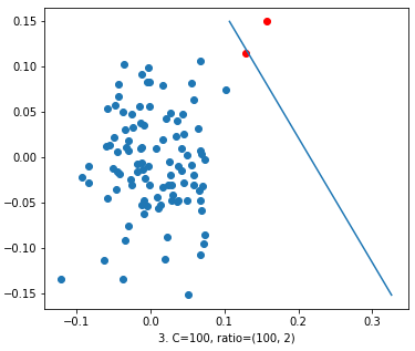
In the 3rd figure, we increased the value of ‘C’ to 100. Here the decision line is trying to classify the red dots from blues. But we can’t say that it’s a good decision function.

Set 2:- Data ratio = (100:20) ->(blue : red)

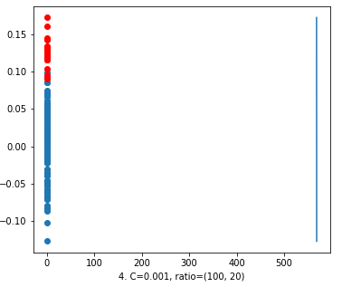
First we look at the value of ‘C’ = 0.001. Comparing the figure 1 and figure 4 will look the same. But looking closely at the x-axis on figure 1, the decision line is at 100k. On the other hand in figure 4, the decision line is at around 600 on x-axis.

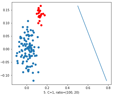
Now, we took the value of ‘C’ = 1. We got a decision line which was very near to the data points but of no use. Because it’s not bifurcating the blues from red.

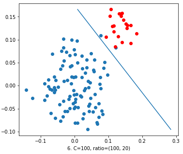
Now, we increased the value of ‘C’ to 100. We can see the resultant figure 6 in which the decision line is well classifying than previous ones. But still it’s not up to mark because the line is near to reds and 2 blues are on the wrong side.

Set 3:- Data ratio = (100:40) ->(blue : red)

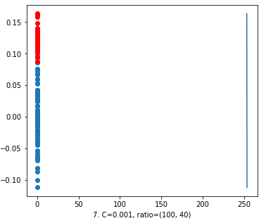
Again we took the value of ‘C’ = 0.001. Like figure 4, in figure 7 also the decision line has moved near to the data points to x-axis. But still it’s useless. No explanation needed.

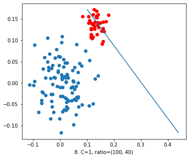
Now, we took the value of ‘C’=1. In figure 8 we can see the decision line trying to classify the data. But it has a lot of errors so, we can’t accept it.

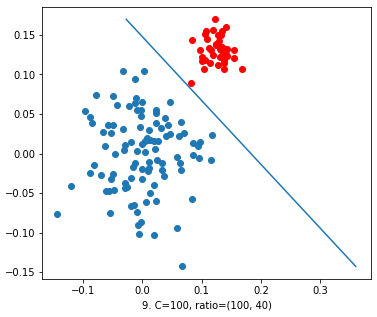
Now, we increased the value of ‘C’ = 100. The decision line has well classified the reds from blues. We can accept this decision function. Thus we can conclude that with this ratio also increasing the value of C will leads us to a good model.

Set 4:- Data ratio = (100:80) ->(blue : red) (almost balanced data set)

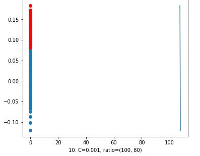
Once again, first we took ‘C’ = 0.001. It is better than the previous model with the same value of ‘C’ but different data ratio. In this model the decision line has come near at 120. So it’s getting better with increased data ratio.

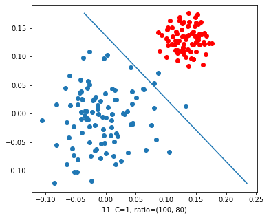
Now we took the value of ‘C’ = 1. In the resultant figure we can observe that the decision is classifying the data. But some blue dots are crossing their boundary. So still there are errors in the model. But obviously it’s getting better.

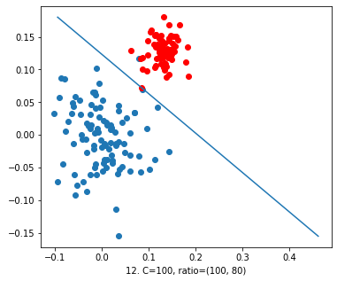
Now moving towards the last figure. We took the value of ‘C’ = 100. In the above figure, we can clearly see a good decision line which is classifying the data well, with an exception. One red and one blue point is exactly on the line. So we can say that it’s a good fit.

Conclusion

From the above observation we can conclude two things.

1. Increasing the data ratio will lead to a better fit of the decision line to data.

2. Increasing the value of ‘C’ will also lead to a good fit of decision line. But after an extent, increasing the it, our model will over fit to the data.

So, train tune your model wisely. !happy coding!