
ICLR 2017 vs arxiv-sanity
I thought it would be fun to cross-reference the ICLR 2017 (a popular Deep Learning conference) decisions (which fall into 4 categories: oral, poster, workshop, reject) with the number of times each paper was added to someone’s library on arxiv-sanity. ICLR 2017 decision making involves a number of area chairs and reviewers that decide the fate of each paper over a period of few months, while arxiv-sanity involves one person working 2 hours once a month (me), and a number of people who use it to tame the flood of papers out there. It is a battle between top down and bottom up. Lets see what happens.
Here are the decisions for ICLR 2017. A total of 491 papers were submitted, of which 15 (3%)will be an oral, 183 (37.3%) a poster, 48 (9.8%)were suggested for workshop and 245 (49.9%) were rejected. The accepted papers will be presented at ICLR on April 24–27 in Toulon, which I am really looking forward to. Look how amazing it looks:

But I digress.
On the other hand we have arxiv-sanity, which has a library feature. In short, any registered user can add a paper to their library, and arxiv-sanity will train a personalized SVM on bigram tfidf features of the full text of all papers to make content-based recommendations to the user. For example, I have a number of RL/generative models/CV papers in my library and whenever there is a new paper on these topics it will come up on top in my “recommended” tab. The review pool of arxiv-sanity is as of now a total of 3195 users — this is the number of people with an account that have at least one paper in the library. Together, these users have so far included 55,671 papers into their libraries, i.e. an average of 17.4 papers.
An important feature of arxiv-sanity is that users don’t just upvote papers with no repercussions. Adding a paper to your library has some weight, because that paper will influence your recommendations. You have an incentive to only include things that really matter to you in there. It’s clever right? No? Okay fine.
The experiment
Long story short, I loop over all papers in ICLR and try to find them on arxiv using an exact match on the title. Some ICLR papers are not on arxiv, and some won’t get matched because the authors renamed them, or they contain weird characters, etc.
For example, lets look at the papers that got an oral at ICLR 2017. We get:
for oral, found 10/15 papers on arxiv with library counts:
 64 Reinforcement Learning with Unsupervised Auxiliary Tasks
 44 Neural Architecture Search with Reinforcement Learning
 38 Understanding deep learning requires rethinking generalizatio...
 28 Towards Principled Methods for Training Generative Adversaria...
 22 Learning End-to-End Goal-Oriented Dialog
 19 Q-Prop: Sample-Efficient Policy Gradient with An Off-Policy C...
 13 Learning to Act by Predicting the Future
 12 Amortised MAP Inference for Image Super-resolution
  8 Multi-Agent Cooperation and the Emergence of (Natural) Langua...
  8 End-to-end Optimized Image Compression
Here we see that we matched 10 out of 15 oral papers on arxiv, and the number next to each one is the number of people who have added that paper to their library. E.g. “Reinforcement Learning with Unsupervised Auxiliary Tasks” was in a library of 64 arxiv-sanity users. I also had to truncate some paper names because medium.com is improperly conceived and doesn’t let you change the font size.
Now lets look at the posters:
for poster, found 113/183 papers on arxiv with library counts:
149 Adversarial Feature Learning
147 Hierarchical Multiscale Recurrent Neural Networks
140 Recurrent Batch Normalization
 80 HyperNetworks
 79 FractalNet: Ultra-Deep Neural Networks without Residuals
 73 Zoneout: Regularizing RNNs by Randomly Preserving Hidden Acti...
 62 Unrolled Generative Adversarial Networks
 52 Adversarially Learned Inference
 49 Quasi-Recurrent Neural Networks
 48 Do Deep Convolutional Nets Really Need to be Deep and Convolu...
 46 Neural Photo Editing with Introspective Adversarial Networks
 43 An Actor-Critic Algorithm for Sequence Prediction
 41 A Learned Representation For Artistic Style
 37 Structured Attention Networks
 33 Mollifying Networks
 30 DeepCoder: Learning to Write Programs
 28 SGDR: Stochastic Gradient Descent with Warm Restarts
 27 Learning to Navigate in Complex Environments
 27 Generative Multi-Adversarial Networks
 26 Soft Weight-Sharing for Neural Network Compression
 25 Pruning Filters for Efficient ConvNets
 24 Why Deep Neural Networks for Function Approximation?
 24 Mode Regularized Generative Adversarial Networks
 24 Dialogue Learning With Human-in-the-Loop
 24 Designing Neural Network Architectures using Reinforcement Le...
 23 PGQ: Combining policy gradient and Q-learning
 22 Frustratingly Short Attention Spans in Neural Language Modeli...
 21 Tracking the World State with Recurrent Entity Networks
 21 Deep Probabilistic Programming
 20 Density estimation using Real NVP
 20 Adversarial Training Methods for Semi-Supervised Text Classif...
 19 Semi-Supervised Classification with Graph Convolutional Netwo...
 19 PixelVAE: A Latent Variable Model for Natural Images
 19 Learning to Optimize
 19 Learning a Natural Language Interface with Neural Programmer
 19 Entropy-SGD: Biasing Gradient Descent Into Wide Valleys
 19 Dynamic Coattention Networks For Question Answering
 18 PixelCNN++: Improving the PixelCNN with Discretized Logistic ...
 18 Generalizing Skills with Semi-Supervised Reinforcement Learni...
 18 Deep Learning with Dynamic Computation Graphs
 18 Automatic Rule Extraction from Long Short Term Memory Network...
 18 Adversarial Machine Learning at Scale
 17 Learning through Dialogue Interactions by Asking Questions
 16 Learning to Perform Physics Experiments via Deep Reinforcemen...
 16 Categorical Reparameterization with Gumbel-Softmax
 15 Sample Efficient Actor-Critic with Experience Replay
 14 Variational Lossy Autoencoder
 14 Identity Matters in Deep Learning
 14 Bidirectional Attention Flow for Machine Comprehension
 13 Towards a Neural Statistician
 13 Recurrent Mixture Density Network for Spatiotemporal Visual A...
 13 On Detecting Adversarial Perturbations
 12 Trained Ternary Quantization
 12 Improving Policy Gradient by Exploring Under-appreciated Rewa...
 12 Capacity and Trainability in Recurrent Neural Networks
 11 SampleRNN: An Unconditional End-to-End Neural Audio Generatio...
 11 Machine Comprehension Using Match-LSTM and Answer Pointer
 11 Latent Sequence Decompositions
 11 Calibrating Energy-based Generative Adversarial Networks
 10 Unsupervised Cross-Domain Image Generation
 10 Learning to Remember Rare Events
 10 Highway and Residual Networks learn Unrolled Iterative Estima...
  9 TopicRNN: A Recurrent Neural Network with Long-Range Semantic...
  9 Steerable CNNs
  9 Query-Reduction Networks for Question Answering
  9 Lossy Image Compression with Compressive Autoencoders
  9 Learning to Compose Words into Sentences with Reinforcement L...
  8 Stick-Breaking Variational Autoencoders
  8 Deep Variational Information Bottleneck
  8 Batch Policy Gradient Methods for Improving Neural Conversati...
  7 Discrete Variational Autoencoders
  7 Data Noising as Smoothing in Neural Network Language Models
  6 Variable Computation in Recurrent Neural Networks
  6 Sigma Delta Quantized Networks
  6 Dropout with Expectation-linear Regularization
  6 Delving into Transferable Adversarial Examples and Black-box ...
  6 A Compositional Object-Based Approach to Learning Physical Dy...
  5 Towards the Limit of Network Quantization
  5 Tighter bounds lead to improved classifiers
  5 Pointer Sentinel Mixture Models
  5 On the Quantitative Analysis of Decoder-Based Generative Mode...
  5 Neuro-Symbolic Program Synthesis
  5 Lie-Access Neural Turing Machines
  5 Learning to superoptimize programs
  5 Learning Features of Music From Scratch
  5 Improving Neural Language Models with a Continuous Cache
  5 Deep Biaffine Attention for Neural Dependency Parsing
  4 Temporal Ensembling for Semi-Supervised Learning
  4 Diet Networks: Thin Parameters for Fat Genomics
  4 DeepDSL: A Compilation-based Domain-Specific Language for Dee...
  4 DSD: Dense-Sparse-Dense Training for Deep Neural Networks
  4 A recurrent neural network without chaos
  3 Trusting SVM for Piecewise Linear CNNs
  3 The Neural Noisy Channel
  3 Revisiting Classifier Two-Sample Tests
  3 Regularizing CNNs with Locally Constrained Decorrelations
  3 Optimal Binary Autoencoding with Pairwise Correlations
  3 Loss-aware Binarization of Deep Networks
  3 Learning Recurrent Representations for Hierarchical Behavior ...
  3 EPOpt: Learning Robust Neural Network Policies Using Model En...
  3 Deep Information Propagation
  2 Words or Characters? Fine-grained Gating for Reading Comprehe...
  2 Topology and Geometry of Half-Rectified Network Optimization
  2 Maximum Entropy Flow Networks
  2 Incorporating long-range consistency in CNN-based texture gen...
  2 Hadamard Product for Low-rank Bilinear Pooling
  1 Multi-view Recurrent Neural Acoustic Word Embeddings
  1 Inductive Bias of Deep Convolutional Networks through Pooling...
  1 Geometry of Polysemy
  1 Autoencoding Variational Inference For Topic Models
  1 A STRUCTURED SELF-ATTENTIVE SENTENCE EMBEDDING
  0 Deep Multi-task Representation Learning: A Tensor Factorisati...
  0 A Compare-Aggregate Model for Matching Text Sequences
Some got a lot of love (149!), and some very little (0). For workshop suggestions we get:
for workshop, found 23/48 papers on arxiv with library counts:
 60 Adversarial examples in the physical world
 31 Learning in Implicit Generative Models
 16 Surprise-Based Intrinsic Motivation for Deep Reinforcement Le...
 14 Multiplicative LSTM for sequence modelling
 13 Efficient Softmax Approximation for GPUs
 12 RenderGAN: Generating Realistic Labeled Data
 12 Generalizable Features From Unsupervised Learning
 10 Programming With a Differentiable Forth Interpreter
  8 Gated Multimodal Units for Information Fusion
  8 Deep Learning with Sets and Point Clouds
  7 Unsupervised Perceptual Rewards for Imitation Learning
  5 Song From PI: A Musically Plausible Network for Pop Music Gen...
  5 Modular Multitask Reinforcement Learning with Policy Sketches
  5 A Differentiable Physics Engine for Deep Learning in Robotics
  4 Exponential Machines
  4 Dataset Augmentation in Feature Space
  3 Semi-supervised deep learning by metric embedding
  2 Adaptive Feature Abstraction for Translating Video to Languag...
  1 Modularized Morphing of Neural Networks
  1 Learning Continuous Semantic Representations of Symbolic Expr...
  1 Extrapolation and learning equations
  0 Online Structure Learning for Sum-Product Networks with Gauss...
  0 Bit-Pragmatic Deep Neural Network Computing
and I won’t list all 200-something papers that were rejected, but lets look at the few that arxiv-sanity users really liked, but the ICLR ACs and reviewers did not:
for reject, found 58/245 papers on arxiv with library counts:
 46 The Predictron: End-To-End Learning and Planning
 39 RL^2: Fast Reinforcement Learning via Slow Reinforcement Lear...
 35 Understanding intermediate layers using linear classifier pro...
 33 Hierarchical Memory Networks
 31 An Analysis of Deep Neural Network Models for Practical Appli...
 20 Low-rank passthrough neural networks
 19 Higher Order Recurrent Neural Networks
 18 Adding Gradient Noise Improves Learning for Very Deep Network...
 16 Unsupervised Pretraining for Sequence to Sequence Learning
 16 A Joint Many-Task Model: Growing a Neural Network for Multipl...
 15 Adversarial examples for generative models
 14 Gated-Attention Readers for Text Comprehension
 13 Extensions and Limitations of the Neural GPU
 12 Warped Convolutions: Efficient Invariance to Spatial Transfor...
 11 Neural Combinatorial Optimization with Reinforcement Learning
 11 Memory-augmented Attention Modelling for Videos
 10 GRAM: Graph-based Attention Model for Healthcare Representati...
  9 Wav2Letter: an End-to-End ConvNet-based Speech Recognition Sy...
  9 Understanding trained CNNs by indexing neuron selectivity
  9 The Power of Sparsity in Convolutional Neural Networks
  9 Improving Stochastic Gradient Descent with Feedback
  8 Towards Information-Seeking Agents
  8 NEWSQA: A MACHINE COMPREHENSION DATASET
  8 LipNet: End-to-End Sentence-level Lipreading
  7 Generative Adversarial Parallelization
  7 Efficient Summarization with Read-Again and Copy Mechanism
  6 Multi-task learning with deep model based reinforcement learn...
  6 Multi-modal Variational Encoder-Decoders
  6 End-to-End Answer Chunk Extraction and Ranking for Reading Co...
  6 Boosting Image Captioning with Attributes
  6 Beyond Fine Tuning: A Modular Approach to Learning on Small D...
  5 Structured Sequence Modeling with Graph Convolutional Recurre...
  5 Human perception in computer vision
  5 Cooperative Training of Descriptor and Generator Networks
Here is the full version, which was not truncated to fit here. There are a few papers on the top of this list that were possibly unfairly rejected.
Here’s another question — what would ICLR 2017 look like if it were simply voted on by the crowd of arxiv-sanity users (of the papers we can find on arxiv)? Here is an excerpt:
oral:
149 Adversarial Feature Learning
147 Hierarchical Multiscale Recurrent Neural Networks
140 Recurrent Batch Normalization
 80 HyperNetworks
 79 FractalNet: Ultra-Deep Neural Networks without Residuals
 73 Zoneout: Regularizing RNNs by Randomly Preserving Hidden Acti...
 64 Reinforcement Learning with Unsupervised Auxiliary Tasks
 62 Unrolled Generative Adversarial Networks
 60 Adversarial examples in the physical world
 52 Adversarially Learned Inference
-------------------------------------------------
poster:
 49 Quasi-Recurrent Neural Networks
 48 Do Deep Convolutional Nets Really Need to be Deep and Convolu...
 46 The Predictron: End-To-End Learning and Planning
 46 Neural Photo Editing with Introspective Adversarial Networks
 44 Neural Architecture Search with Reinforcement Learning
 43 An Actor-Critic Algorithm for Sequence Prediction
 41 A Learned Representation For Artistic Style
 39 RL^2: Fast Reinforcement Learning via Slow Reinforcement Lear...
 38 Understanding deep learning requires rethinking generalizatio...
 37 Structured Attention Networks
 35 Understanding intermediate layers using linear classifier pro...
 33 Mollifying Networks
 33 Hierarchical Memory Networks
 31 Learning in Implicit Generative Models
 31 An Analysis of Deep Neural Network Models for Practical Appli...
 30 DeepCoder: Learning to Write Programs
...
Again, the full listing can be found here. Note that in particular, some ICLR2017 papers that were rejected would have been almost an oral based on arxiv-sanity users alone, especially the Predictron, RL², “Understanding intermediate layers”, and “Hierarchical Memory Networks”. Conversely, some accepted papers had very little love from arxiv-sanity users. Here is a full confusion matrix:
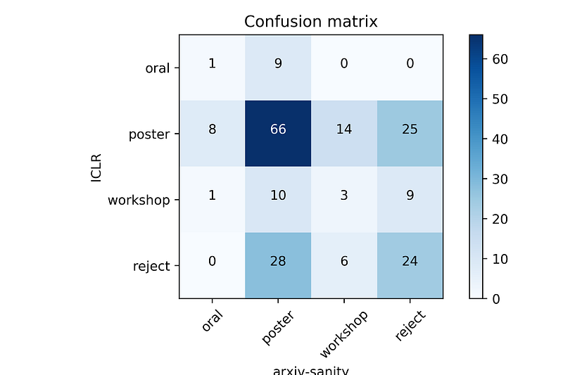
And here is the confusion matrix in text, for each cell, together with the paper titles. This doesn’t look too bad. The two groups don’t agree on the orals at all, agree on the posters quite a bit, and most importantly there are very few confusions between oral/poster and rejection. Also, congratulations to Max et al. for “Reinforcement Learning with Unsupervised Auxiliary Tasks”, which is the only paper that both groups agree should be an oral :)
Finally, I read the following Medium post a few days ago: “Ten Deserving Deep Learning Papers that were Rejected at ICLR 2017”, by Carlos E. Perez. It seems that arxiv-sanity users agree with this post, and all papers listed there (including LipNet)(that we could also find on arxiv) would have been accepted by arxiv-sanity users.
Discussion
An asterisk. There are several factors that skew these results. For example, the size of arxiv-sanity user base grows over time, so these results likely slightly favor papers that were published on arxiv later than earlier, as these would have come to more user’s attention as new papers on the site. Also, papers are not seen with equal frequencies — for instance if some paper gets tweeted out by someone popular, more people will see it, and more people might add it to their library. And finally, a good argument could be made that on arxiv-sanity “rich get richer”, because arxiv papers are not anonymous and celebrities could get more attention. In this particular case, ICLR 2017 is single-blind so this is not a differentiating factor.
Overall, my own conclusion from this experiment is that there is quite a bit of signal here. And we’re getting it “for free” from a bottom up process on the internet, instead of something that takes a few hundred people several months. And as someone who has had a good amount of long, painful, stressful, rebuttals back and forth on both submitting/reviewing sides that dragged on for multiple weeks/months, I say: Maybe we don’t need it. Or at the very least maybe there is a lot of room for improvement.
EDIT1: someone suggested the fun idea that we add up the number of citations of these papers in ICLR 2018 submitted/accepted papers, and see which ranking “wins” on that metric. Looking forward to that :)