
Hypothesis Testing #9 — Kruskal-Wallis Test using R
The Kruskal-Wallis test is a non-parametric test that compares two or more samples to determine whether their median values are significantly different. It is an extension of the Mann-Whitney U test, which is used for comparing only two samples. This test is mainly used in scenarios where we identify potential dissimilarities between the median values of different groups, but these data points from the samples do not form a normal distribution.
The test is named after American statisticians William Kruskal and W. Allen Wallis.

Table of Content
· Kruskal-Wallis Test ∘ Installation ∘ R Script ∘ Explanation of the kruskal.test function in R ∘ p-value Intrepretation · Note
Assuming you have installed RStudio Desktop…
Kruskal-Wallis Test
Installation
# The Kruskal-Wallis Test is a built-in function within R. Hence, no installation is required.The Kruskal-Wallis Test within R has the following code:
R Script
getAnywhere(kruskal.test.default)function (x, g, ...)
{
if (is.list(x)) {
if (length(x) < 2L)
stop("'x' must be a list with at least 2 elements")
if (!missing(g))
warning("'x' is a list, so ignoring argument 'g'")
DNAME <- deparse1(substitute(x))
x <- lapply(x, function(u) u <- u[complete.cases(u)])
if (!all(sapply(x, is.numeric)))
warning("some elements of 'x' are not numeric and will be coerced to numeric")
k <- length(x)
l <- lengths(x)
if (any(l == 0L))
stop("all groups must contain data")
g <- factor(rep.int(seq_len(k), l))
x <- unlist(x)
}
else {
if (length(x) != length(g))
stop("'x' and 'g' must have the same length")
DNAME <- paste(deparse1(substitute(x)), "and", deparse1(substitute(g)))
OK <- complete.cases(x, g)
x <- x[OK]
g <- g[OK]
g <- factor(g)
k <- nlevels(g)
if (k < 2L)
stop("all observations are in the same group")
}
n <- length(x)
if (n < 2L)
stop("not enough observations")
r <- rank(x)
TIES <- table(x)
STATISTIC <- sum(tapply(r, g, sum)^2/tapply(r, g, length))
STATISTIC <- ((12 * STATISTIC/(n * (n + 1)) - 3 * (n + 1))/(1 -
sum(TIES^3 - TIES)/(n^3 - n)))
PARAMETER <- k - 1L
PVAL <- pchisq(STATISTIC, PARAMETER, lower.tail = FALSE)
names(STATISTIC) <- "Kruskal-Wallis chi-squared"
names(PARAMETER) <- "df"
RVAL <- list(statistic = STATISTIC, parameter = PARAMETER,
p.value = PVAL, method = "Kruskal-Wallis rank sum test",
data.name = DNAME)
class(RVAL) <- "htest"
return(RVAL)
}Explanation of the kruskal.test function in R
Let’s break the code down line by line.
- If
xis not a list or if the length ofxis less than 2, stop and display an error message stating thatxmust be a list with at least 2 elements. - If
xis a list and thegargument in the function is provided, issue a warning stating thatxis a list and the 'g' argument will be ignored. - Deparse the name of
xintoDNAME. - Ensure that all elements in the list
xare non-empty. - If any elements of
xare not numeric, issue a warning that non-numeric elements will be coerced to numeric. - Calculate the count of elements in
xand store it in the variablek. This represents the number of levels in factors, for example. - Sum the total number of values across all elements in
xand store this in the variablel. - If any value in
lis 0, stop and display an error message stating that all groups must contain data. - Create a factor
gby repeating the numbers 1 tok, each a number of times specified byl, which is useful for generating categorical group identifiers. - Unlist
xand reassign it back tox. - If
xis not a list and the length ofxdoes not equal the length ofg, stop and display an error message stating thatxandgmust have the same length. - Combine and deparse the names of
xandgintoDNAME. - Identify all complete cases for
xandgand retain these indices. - Filter out empty values from
xandg. - Re-factorize
gand assign it back tog. - Determine the number of levels in
gand store this ink. - If
kis less than 2, stop and display an error message stating that all observations are in the same group. - Calculate the total number of values in
xand store this inn. - If
nis less than 2, stop and display an error message stating there are not enough observations. - Rank all values in
x, assigning the smallest value the rank of 1, and store these ranks inr. - Create a frequency table of
xvalues and store it in the variableTIES. - Calculate the test statistic: sum the squared ranks within each group, divide by the group sizes, and sum these values. Store this in
STATISTIC. - Refine
STATISTICby multiplying it by 12, dividing byn * (n + 1), subtracting3 * (n + 1), and then dividing by1 - (sum(TIES^3 - TIES) / (n^3 - n)). - Set
PARAMETERtok - 1. - Calculate the p-value using the
pchisqfunction withSTATISTIC,PARAMETER, andlower.tail = FALSEfor upper tail probability in hypothesis testing. - Label
STATISTICas 'Kruskal-Wallis chi-squared' andPARAMETERas 'df'. - Create a list
RVALcontainingSTATISTIC,PARAMETER,PVAL,method = 'Kruskal-Wallis rank sum test', andDNAME. - Set the class of
RVALto 'htest'.
Things to take note:
- The values will be converted into ordinal factors, meaning that they are considered as groupings with meaningful levels or intervals.
- In point 23, there are four major mathematical operations. First, we want to scale the STATISTIC to conform to the chi-squared distribution. We achieve this by multiplying it by 12. Please refer to the note here for an explanation of why 12 is used.
- The Kruskal-Wallis test utilizes the chi-squared distribution to assess the null hypothesis, which often pertains to the equality of medians across groups. The effectiveness, or statistical power, of this test is influenced by sample size. Specifically, with a smaller sample size, the test has a higher likelihood of committing a Type II error, meaning it may fail to detect a true difference when one actually exists. In contrast, larger sample sizes generally increase the test’s power, reducing the probability of a Type II error.
- The test checks whether one sample is greater than the other. Therefore, the lower.tail is set to FALSE as we want the upper tail.
Let’s generate some random data as an example:
# Set seed for reproducibility
set.seed(9876)

# Generate sample data with similar group means
group1 <- rnorm(50, mean = 10, sd = 1)  # Normal distribution with mean 10
group2 <- rnorm(50, mean = 10.2, sd = 1)  # Normal distribution with mean 10.2
group3 <- rnorm(50, mean = 10.1, sd = 1)  # Normal distribution with mean 10.1

# Combine data into a single data frame
data <- data.frame(
  value = c(group1, group2, group3),
  group = factor(rep(c("Group 1", "Group 2", "Group 3"), each = 50))
)
We execute the test:
# Perform Kruskal-Wallis test
result <- kruskal.test(value ~ group, data = data)
We get the following result:
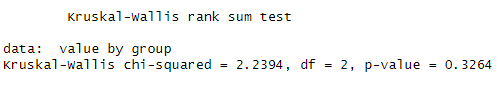
Graphically, we have the following:
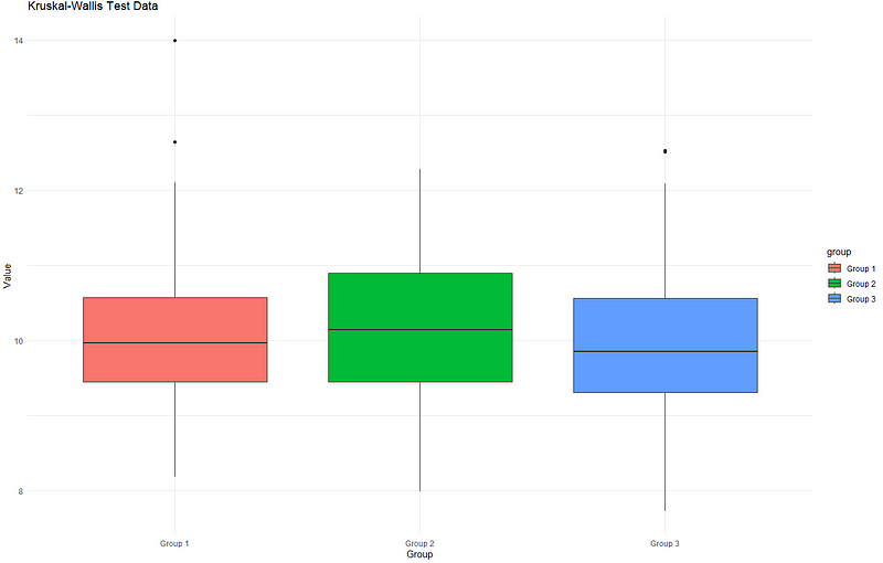
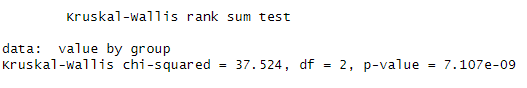
Notice that the median values for the groups are not far apart from each other, resulting in a p-value greater than 0.05. Now, if we add more noise to it, you will see that the median values are no longer similar. We generate another set of random data, but this time we have differing median values and varying standard deviations.
We get the following result:
If we plot the graph:
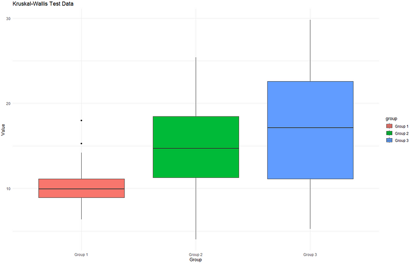
As you may have observed, the median values are significantly different. Additionally, the variation varies among each group, which can be observed by the size of the box.
p-value Intrepretation
Null hypothesis: There is no significant difference among the medians of the different groups being compared. In other words, it assumes that all groups are samples from the same population or distribution.
Alternative hypothesis: There is a significant difference among the medians of at least two of the groups being compared.
When the p-value is 0.05 or lower, we reject the null hypothesis, indicating a significant difference in the median values between two or more groups. If there is insufficient evidence to reject the null hypothesis, we conclude that there is no significant difference between the median values of the groups.

Daniel began his career as a senior list researcher with a British publishing firm. At that time, his role involved sourcing contacts through the internet and performing data entry into the Microsoft Dynamic CRM system (Microsoft Dynamic CRM 3.0). Gradually, he explored the option of using Visual Basic scripting within Excel to automate the contact sourcing process. He successfully developed and implemented scripts, leading to a 95% increase in data entry efficiency. He then transitioned to the role of a CRM executive with Fuji Xerox Singapore.
As a CRM executive, he liaised with a third-party vendor for technical enhancement of the CRM system (Microsoft Dynamic CRM 4.0 and 365) and performed functional enhancements for hundreds of end users. His notable achievement was the development of the CRM bot, which led to a 98% improvement in data quality and integrity in the CRM system. Following his Master’s studies in Consumer Insight at Nanyang Business School, he became an Analytics instructor at Singapore Management University. He prepared class notes and technical walkthroughs and taught Analytics to undergraduate students from various disciplines. He then took on various consulting roles in the consultancy, manufacturing, and information technology industries in Singapore.

He traveled to Paris, London, Sri Lanka, Japan, and Malaysia to fulfill his consulting roles. The cultural and professional exchanges between local and overseas data analysts gave him a comprehensive overview of expectations and motivations from people around the world. He also had the opportunity to relocate to the United States for one year, focusing on Operations Management.
Before becoming a business owner, he was the Data Science Lead in a Singaporean software company. His primary role involved developing Artificial Intelligence using logic, data science, and machine learning techniques through in-depth, full-stack scripting. He also developed customized reporting for his customers, believing that 95% of today’s reporting could be automated, which would free up staff from daily manual work.

He holds a Bachelor of Science in Marketing (BSc. Marketing, Pass with Merit) from the Singapore University of Social Sciences, where he graduated as Valedictorian, a Master of Science in Marketing and Consumer Insights (MSc. Marketing and Consumer Insights) from Nanyang Technological University, and a Doctor of Business Administration (DBA) from the Swiss School of Business and Management.
Note
We rank each observation across all groups. If there are N observations in total, these ranks are uniformly distributed from 1 to N.
Now, the mean value of the uniform distribution is:

We calculate the variance of the uniform distribution:

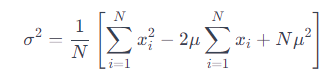
We further expand it into the variance formula:
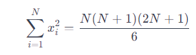
We find the sum of the squares of the first N natural numbers:
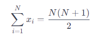
We find the sum of the first N natural numbers:
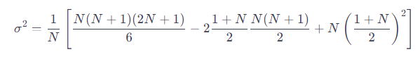
We substitute the previous two formulas into the variance formula:
We simply the equation to arrive at:


