
Hypothesis Testing #6 — Bayesian Analysis using Cauchy Distribution
Table of Content
· Bayesian Analysis · Prior Belief · Likelihood · Posterior Probability · R Script

Bayesian Analysis
The Bayesian Analysis is an alternative to the frequentist style of analysis. Before I lose you, allow me to explain a little.
Here are the differences:
- Frequentist: The probability of events is derived from how often these events have occurred or are expected to occur. The focus is on these events and modelling them based on observed data. [Bayesian: Here, the probability of events is based on prior beliefs or assumptions. We start with these beliefs and then update them with new data, leading to a revised probability. This process is like taking an initial belief (A), applying new evidence, and arriving at a new belief (B).]
- Frequentist: In this approach, the available data is used to determine the parameters that describe the events. These parameters assist in shaping our understanding and models of the data. It’s akin to continually generating new models as time progresses. [Bayesian: In Bayesian analysis, parameters are treated as random variables. The transition from one belief (prior) to another (posterior) is guided by the data we analyze. The initial belief (prior) is updated to become the posterior belief in light of new evidence, and this posterior belief then serves as the new prior belief for subsequent analysis.]
- Frequentist: This approach heavily relies on hypothesis testing, using confidence levels and test statistics to make inferences. [Bayesian: No test statistic is involved, and testing is based on the calculation of probabilities. Bayesian analysis uses prior knowledge or beliefs, which are updated with the available data to make inferences. This approach calculates the probability of a hypothesis being true given the observed data.]
In short, Bayesian analysis refers to the process of updating an initial belief with new evidence, leading to a revised belief. This process can be recursive as new evidence emerges. Then, what about the Cauchy Distribution? Please visit this discussion where I have briefly explained the Cauchy distribution in simple terms.
When performing Bayesian analysis with the Cauchy Distribution, we first consider our prior belief.
Prior Belief
In Bayesian analysis using the Cauchy Distribution, we assume that our prior belief adheres to this distribution. Imagine we have a set of data and the data fits the Cauchy Distribution, the probability values arising from the distribution form the prior of the Bayesian analysis.
The Cauchy Distribution is characterized by its location parameter, representing the median of the data, and its scale parameter, which determines the spread of the distribution curve. Therefore, establishing these parameters is a critical first step in deriving the probabilities for prior belief.
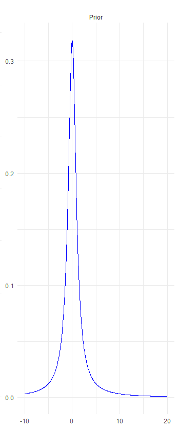
Note that the x-axis of the Cauchy distribution represents real values, which can include zero or negative numbers. The y-axis indicates the density or ‘popularity’ at a given point on the x-axis. This is a probability density function curve. When calculating the area under the curve of the Cauchy distribution, it sums up to 1, representing the entire probability space of the sample.
The next step is to consider the Likelihood.
Likelihood
Likelihood is the new evidence used to revise your prior belief. Imagine it as dropping a dense object into a small bathtub: the water in the bathtub represents your initial belief. When a new object is introduced, the water level rises. This new water level is analogous to your posterior probability, which I will explain shortly.
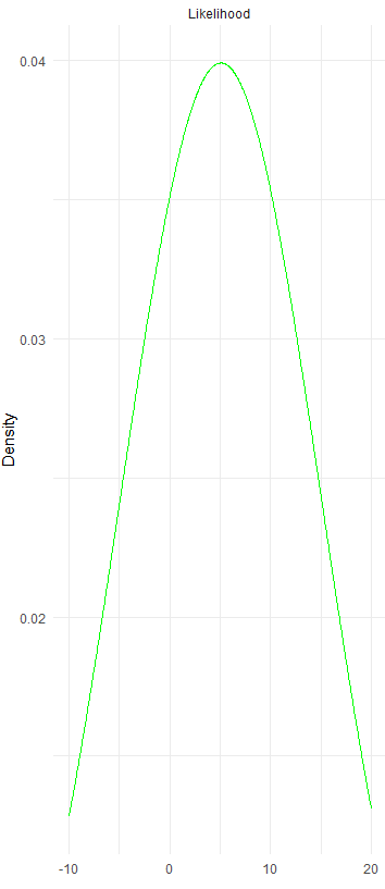
The likelihood doesn’t necessarily need to follow the same distribution as the prior belief. This makes intuitive sense, as distributions can change over time. Therefore, we cannot always expect the distribution used for the prior belief to be the same as that for the likelihood, which reflects events or observations that occur or are observed later. We calculate the likelihood based on the specific distribution that is most appropriate for the new evidence or data.
Posterior Probability
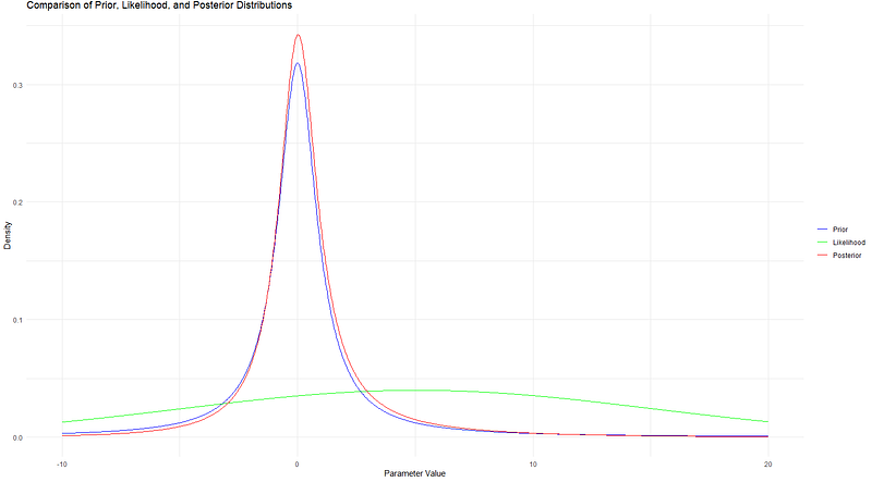
The posterior probability represents the updated belief that you adopt after adjusting the prior belief with the likelihood. Let’s examine what the posterior probability looks like.
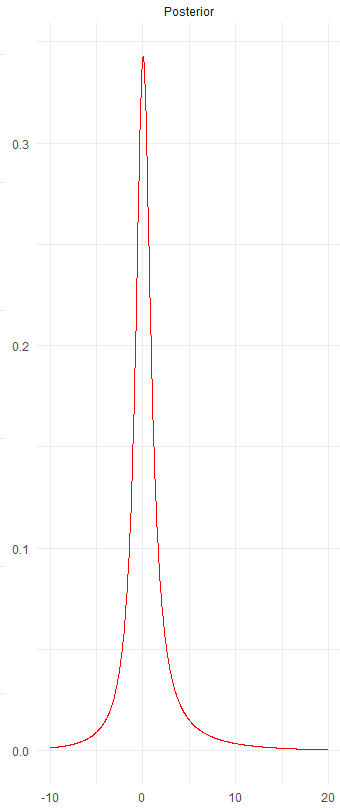
When comparing the prior belief to the posterior probabilities, you’ll often observe that the posterior probabilities have a slightly higher peak. This happens because the likelihood probabilities modify the prior probabilities, leading to the formation of the posterior probabilities. We understand that prior probabilities are calculated using the probability density function of the Cauchy distribution. Similarly, the likelihood is derived from a distribution, which may not be the same as that used for the prior probabilities. Now, the question arises: How exactly do we calculate the posterior probability?
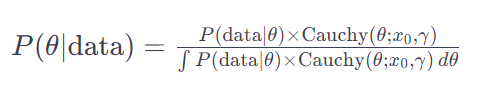
Let’s understand this formula closer:
The numerator is a product of the likelihood and the prior. The denominator is a tough nut to crack.
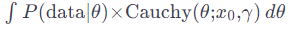
Assuming we have our numerator, which is the product of the prior and likelihood distributions, the output can be seen as a combination of two different distributions, particularly if the likelihood distribution differs from the prior. Imagine this process as a recipe that blends apples and oranges. It’s not enough to just mix these ingredients; we need to ensure that their combination results in a harmonious dish. This is where normalization, involving the denominator, comes into play. The numerator combines the ingredients (distributions), but it’s the denominator that ensures the resulting mixture is balanced and palatable, much like achieving the right balance of flavors in a culinary dish.
R Script
Assuming you have installed RStudio Desktop…
In an R script, the prior is computed based on the relevant probability density function, which in this scenario is the Cauchy distribution. Similarly, the likelihood distribution is calculated according to its respective probability density function. The following R script demonstrates how to calculate the posterior distribution by combining these elements:
posterior_function <- function(x) prior_function(x) * likelihood_function(x)
posterior_values <- posterior_function(x_values)
posterior_integral <- sum(posterior_values * diff(c(x_values[1], x_values))) # Numerical integration
posterior <- posterior_values / posterior_integral
The first line of the script defines a new posterior function as the product of the prior function and the likelihood function, where each of these functions represents the respective probability density functions of the data.
The second line generates the posterior values, which are computed as the product of each corresponding prior value and its respective likelihood value.
The third line sums all the product of the individual posterior values with the difference between consecutive elements in the x_values array. It's used to approximate the width of each segment for numerical integration. By appending x_values[1] at the beginning, it ensures the array used in the difference calculation has the same length as the original x_values, providing a width for each interval.
The final line of the script computes the definitive posterior values. It’s important to note that these posterior values are initially generated as a product of the prior and likelihood values. They are then adjusted through numerical integration to obtain the final, normalized posterior values. This process completes the Bayesian analysis using the Cauchy Distribution as the prior.

Daniel started off his career as a senior list researcher with a British publishing firm. Back then, his role involved contact sourcing through the internet and performed data entry into the Microsoft Dynamic CRM system. (Microsoft Dynamic CRM 3.0) Progressively, he explored the option of using Visual Basic scripting within excel to automate the contact sourcing process.
He successfully developed and implemented the scripts, leading to 95% increase in data entry efficiency. He then moved on to take on the role of a CRM executive with Fuji Xerox Singapore.
As a CRM executive, he liaised with third party vendor for technical enhancement of the CRM system (Microsoft Dynamic CRM 4.0 and 365). He also performs functional enhancement of the CRM system for hundreds of end users.
His notable achievement was the development of the CRM boy that led to 98% improvement in data quality and data integrity in the CRM system. Following his Masters studies in Consumer Insight with Nanyang Business School, he took on the role of an Analytics instructor with Singapore Management University. He prepared class notes and technical walkthrough, and taught Analytics to the undergraduate students from various disciplines. Subsequently, he took on various roles as consultants in the consultancy, manufacturing and information technology industries in Singapore.

He travelled to Paris, London, Sri Lanka, Japan and Malaysia to fulfill his role as a consultant. The cultural and professional exchanges between local and overseas data analytics had given him a very good overview of the expectations and motivations from people around the world. He also had a chance to relocate to the United States for one year, particularly focusing on Operations Management.
Prior to his current freelance status, he took on the role of the Data Science Lead in a Singaporean software company. His primary role was to develop Artificial Intelligence using logic, data science and machine learning techniques through in-depth, full-stacked scripting. He also developed customized Reporting for his customers. In his point of view, 95% of today’s reporting can be automated, which can free up staff from daily manual work.

He holds a Bachelor of Science in Marketing (BSc. Marketing Pass with Merit) from Singapore University of Social Sciences (in which he graduated as a Valedictorian), a Master of Science in Marketing and Consumer Insights (MSc. Marketing and Consumer Insights) from Nanyang Technological University, a Doctor of Business Administration (DBA) from Swiss School of Business and Management.