Hypothesis Testing #1b — Kolmogorov-Smirnov Test (K-S Test) using R

The Normality Test is a test to determine whether the sample data is drawn from a normally distributed population. There are several tests available for this purpose. We will look at each one in detail.

Assuming you have installed RStudio Desktop…

Kolmogorov-Smirnow Test (K-S Test)

I’ll use the term K-S Test from now on.

The K-S Test was named after two Russian statisticians from the era of the Russian Empire, Andrey Kolmogorov and Nikolai Smirnov. It was introduced in the 1930s, before World War II broke out. During that time, Joseph Stalin, who became the leader of the Soviet Union, imposed strict censorship on academic research and publication. Given this context, it is likely that both statisticians were sufficiently loyal to the Russian Empire, allowing their research work to proceed unhindered. This is noteworthy, considering many academics and scholars were executed for anti-Soviet activities. Successfully having a test accepted, adopted, and named after them was a significant achievement in those days.

# The Shapiro-Wilk Test is a built-in function within R. Hence, no installation is required.

The K-S Test within R has the following code:

ks.test

function (x, y, ..., alternative = c("two.sided", "less", "greater"), 
    exact = NULL, simulate.p.value = FALSE, B = 2000) 
{
    alternative <- match.arg(alternative)
    DNAME <- deparse1(substitute(x))
    x <- x[!is.na(x)]
    n <- length(x)
    if (n < 1L) 
        stop("not enough 'x' data")
    PVAL <- NULL
    if (is.ordered(y)) 
        y <- unclass(y)
    if (is.numeric(y)) {
        args <- list(...)
        if (length(args) > 0L) 
            warning("Parameter(s) ", paste(names(args), collapse = ", "), 
                " ignored")
        DNAME <- paste(DNAME, "and", deparse1(substitute(y)))
        y <- y[!is.na(y)]
        n.x <- as.double(n)
        n.y <- length(y)
        if (n.y < 1L) 
            stop("not enough 'y' data")
        if (is.null(exact)) 
            exact <- (n.x * n.y < 10000)
        if (!simulate.p.value) {
            METHOD <- paste(c("Asymptotic", "Exact")[exact + 
                1L], "two-sample Kolmogorov-Smirnov test")
        }
        else {
            METHOD <- "Monte-Carlo two-sample Kolmogorov-Smirnov test"
        }
        TIES <- FALSE
        n <- n.x * n.y/(n.x + n.y)
        w <- c(x, y)
        z <- cumsum(ifelse(order(w) <= n.x, 1/n.x, -1/n.y))
        if (length(unique(w)) < (n.x + n.y)) {
            z <- z[c(which(diff(sort(w)) != 0), n.x + n.y)]
            TIES <- TRUE
            if (!exact & !simulate.p.value) 
                warning("p-value will be approximate in the presence of ties")
        }
        STATISTIC <- switch(alternative, two.sided = max(abs(z)), 
            greater = max(z), less = -min(z))
        nm_alternative <- switch(alternative, two.sided = "two-sided", 
            less = "the CDF of x lies below that of y", greater = "the CDF of x lies above that of y")
        z <- NULL
        if (TIES) 
            z <- w
        PVAL <- switch(alternative, two.sided = psmirnov(STATISTIC, 
            sizes = c(n.x, n.y), z = w, exact = exact, simulate = simulate.p.value, 
            B = B, lower.tail = FALSE), less = psmirnov(STATISTIC, 
            sizes = c(n.x, n.y), , z = w, exact = exact, simulate = simulate.p.value, 
            B = B, two.sided = FALSE, lower.tail = FALSE), greater = psmirnov(STATISTIC, 
            sizes = c(n.x, n.y), , z = w, exact = exact, simulate = simulate.p.value, 
            B = B, two.sided = FALSE, lower.tail = FALSE))
        if (simulate.p.value) 
            PVAL <- (1 + (PVAL * B))/(B + 1)
    }
    else {
        if (is.character(y)) 
            y <- get(y, mode = "function", envir = parent.frame())
        if (!is.function(y)) 
            stop("'y' must be numeric or a function or a string naming a valid function")
        TIES <- FALSE
        if (length(unique(x)) < n) {
            warning("ties should not be present for the Kolmogorov-Smirnov test")
            TIES <- TRUE
        }
        if (is.null(exact)) 
            exact <- (n < 100) && !TIES
        METHOD <- paste(c("Asymptotic", "Exact")[exact + 1L], 
            "one-sample Kolmogorov-Smirnov test")
        x <- y(sort(x), ...) - (0:(n - 1))/n
        STATISTIC <- switch(alternative, two.sided = max(c(x, 
            1/n - x)), greater = max(1/n - x), less = max(x))
        if (exact) {
            PVAL <- 1 - if (alternative == "two.sided") 
                .Call(C_pKolmogorov2x, STATISTIC, n)
            else {
                pkolmogorov1x <- function(x, n) {
                  if (x <= 0) 
                    return(0)
                  if (x >= 1) 
                    return(1)
                  j <- seq.int(from = 0, to = floor(n * (1 - 
                    x)))
                  1 - x * sum(exp(lchoose(n, j) + (n - j) * log(1 - 
                    x - j/n) + (j - 1) * log(x + j/n)))
                }
                pkolmogorov1x(STATISTIC, n)
            }
        }
        else {
            PVAL <- if (alternative == "two.sided") 
                1 - .Call(C_pKS2, sqrt(n) * STATISTIC, tol = 1e-06)
            else exp(-2 * n * STATISTIC^2)
        }
        nm_alternative <- switch(alternative, two.sided = "two-sided", 
            less = "the CDF of x lies below the null hypothesis", 
            greater = "the CDF of x lies above the null hypothesis")
    }
    names(STATISTIC) <- switch(alternative, two.sided = "D", 
        greater = "D^+", less = "D^-")
    PVAL <- min(1, max(0, PVAL))
    RVAL <- list(statistic = STATISTIC, p.value = PVAL, alternative = nm_alternative, 
        method = METHOD, data.name = DNAME, data = list(x = x, 
            y = y), exact = exact)
    class(RVAL) <- c("ks.test", "htest")
    return(RVAL)
}

With the help of GPT4.0, let’s break it down slowly.

1. Function Parameters:

• x, y: The data vectors.
• alternative: Specifies the alternative hypothesis. The options are "two.sided", "less", or "greater".
• exact: A logical value indicating whether to use the exact distribution of the test statistic.
• simulate.p.value: A boolean for whether to simulate the p-value.
• B: Number of bootstrap replicates for p-value computation.

2. Initial Checks and Preparations:

• It checks if x or y have sufficient data after removing NA values.
• It checks if y is a numeric vector or a function.
• It sets the method of calculation based on the exact and simulate.p.value flags.

3. Handling Ties:

• The code accounts for ties (duplicate values) in the data, which can affect the KS test.

4. Calculation of Test Statistic:

• For a two-sample test, the test statistic is computed based on the cumulative distributions of x and y.
• For a one-sample test, the test statistic is computed based on the cumulative distribution of x and the specified distribution function y.

5. P-Value Calculation:

• Depending on the method (exact, asymptotic, or Monte-Carlo simulation), the p-value is calculated differently.
• For the exact calculation, it uses custom functions or in-built R functions.
• If simulate.p.value is true, it simulates the p-value using bootstrap methods.

6. Result Preparation:

• The result includes the test statistic, p-value, description of the alternative hypothesis, the method used, and the data names.
• The result is formatted as an object of class ks.test and htest.

In this function, we observed some rules:

1. While the function handles the emptiness of the variable, at the final preparation where the variables contain non-empty values, the number of values should be sufficiently large and not 1 or 2.
2. If the same values exist in variables such as a tie, the p-value will be approximated.

Let’s generate some random data as an example:

Two-Sample Test

set.seed(98765)

# Generate first dataset (e.g., normal distribution)
mean1 <- 5
sd1 <- 1
size1 <- 100
data1 <- rnorm(size1, mean = mean1, sd = sd1)

# Generate second dataset with a different distribution (e.g., uniform distribution)
min2 <- 3
max2 <- 7
size2 <- 100
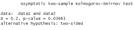
data2 <- runif(size2, min = min2, max = max2)

We execute the script

ks_test_result <- ks.test(data1, data2)

and the result:

One-Sample Test (Test against a theoretical distribution)

set.seed(98765)

# Generate a dataset (e.g., from a normal distribution)
mean_sample <- 0
sd_sample <- 1
size_sample <- 100
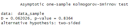
data_sample <- rnorm(size_sample, mean = mean_sample, sd = sd_sample)

We execute the script

ks_test_result <- ks.test(data_sample, "pnorm", mean = 0, sd = 1)

and the result:

Comparing two samples is the limit; we cannot compare three or more samples unless we resort to pairwise comparisons. In our current discussion, our primary interest lies in determining whether a sample follows normality. Therefore, we are using the one-sample test in our analysis.

Let’s study the ‘D’ value a little closer.

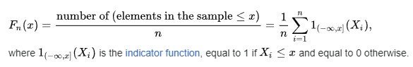
The indicator function is a crucial component of the K-S Test. It checks all possible data points, starting from the lowest value. Moving upward from this lowest value, at each point, the function evaluates if there are any values in the dataset that are less than or equal to the current data point. If, for example, there are 10 values in your dataset that are lower or equal to this data point, then you take 10 divided by the total number of values in the dataset. This function’s value will always be 1 or less.

Let’s consider a numerical example. Suppose we have the prices of Apple MacBooks, ranging from the lowest at US$700 to the highest at US$2,000. Our data includes:

• MacBook 1: US$700
• MacBook 2: US$950
• MacBook 3: US$1,100
• MacBook 4: US$1,200
• MacBook 5: US$1,500
• MacBook 6: US$1,750
• MacBook 7: US$1,880
• MacBook 8: US$1,920
• MacBook 9: US$1,999
• MacBook 10: US$2,000

The steps are as follows:

1. Start with the value 0, the lowest possible price. No MacBooks are priced at or below 0.
2. Move to 1. Again, no MacBooks are priced at or below 1.
3. Continue this process up to US$699.
4. At US$700, there is one MacBook priced at or below this value. Hence, at US$700, we take 1 MacBook divided by the total, which is 10.
5. Proceed to US$701. Only one MacBook is priced at or below US$701, so the calculation remains 1 divided by 10.
6. Fast forward to US$949.
7. At US$950, there are two MacBooks priced at or below this value. Now, we take 2 MacBooks divided by the total, which is 10.
8. Continue this process.

When we reach the highest value, US$2,000, the proportion will have reached 1. Statistically, this is known as the empirical distribution, a type of cumulative distribution.

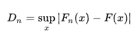
Now, once we have this empirical distribution, we compare it with the theoretical, ideally normal distribution, assuming all the values fall perfectly within the distribution. We use a ruler to compare vertically between the two distributions (the empirical and the normal distributions). The greatest distance between these two distributions is our test statistic. This test statistic is then compared to the Kolmogorov distribution.

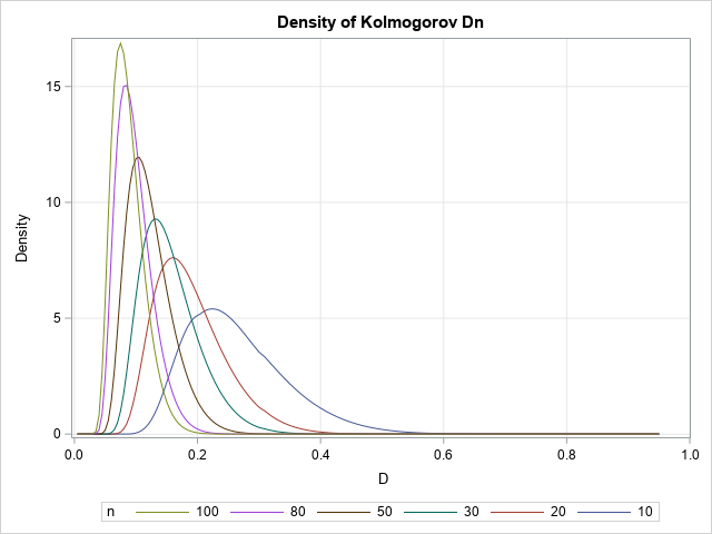
The test statistic will always be 1 or below. Since it compares the cumulative curves, the vertical distance between two cumulative curves will always be 1 or less.

p-value Interpretation

The p-value in the K-S Test is derived from the Kolmogorov Distribution, as shown above. We use this p-value to decide whether to reject the null hypothesis.

Null Hypothesis: The null hypothesis states that the sample data comes from the specified theoretical distribution. For instance, if you are comparing your sample data to a normal distribution, H0 posits that your data follows a normal distribution.

Alternative Hypothesis (H1): The alternative hypothesis states that the sample data does not come from the specified theoretical distribution. Continuing with the normal distribution example, H1 would suggest that your data does not follow a normal distribution.

In statistical analyses, especially when evaluating normality with tests such as the Kolmogorov-Smirnov Test, understanding p-values and the D statistic is essential.

A p-value, representing the probability of observing data as extreme as the sample under the null hypothesis, is crucial for hypothesis testing. A low p-value (usually less than 0.05) suggests strong evidence against the null hypothesis, indicating that the data likely does not follow a normal distribution. On the other hand, a high p-value implies insufficient evidence to reject the null hypothesis, suggesting the data might be normally distributed. The D statistic, integral to these tests, measures the maximum distance between the empirical distribution function and the theoretical distribution. A higher D statistic typically corresponds to a lower p-value, indicating a greater deviation from normality, while a lower D statistic is associated with a higher p-value, suggesting closer adherence to a normal distribution.

Dr. Daniel Koh

Daniel started off his career as a senior list researcher with a British publishing firm. Back then, his role involved contact sourcing through the internet and performed data entry into the Microsoft Dynamic CRM system. (Microsoft Dynamic CRM 3.0) Progressively, he explored the option of using Visual Basic scripting within excel to automate the contact sourcing process.

He successfully developed and implemented the scripts, leading to 95% increase in data entry efficiency. He then moved on to take on the role of a CRM executive with Fuji Xerox Singapore.

As a CRM executive, he liaised with third party vendor for technical enhancement of the CRM system (Microsoft Dynamic CRM 4.0 and 365). He also performs functional enhancement of the CRM system for hundreds of end users.

His notable achievement was the development of the CRM boy that led to 98% improvement in data quality and data integrity in the CRM system. Following his Masters studies in Consumer Insight with Nanyang Business School, he took on the role of an Analytics instructor with Singapore Management University. He prepared class notes and technical walkthrough, and taught Analytics to the undergraduate students from various disciplines. Subsequently, he took on various roles as consultants in the consultancy, manufacturing and information technology industries in Singapore.

He travelled to Paris, London, Sri Lanka, Japan and Malaysia to fulfill his role as a consultant. The cultural and professional exchanges between local and overseas data analytics had given him a very good overview of the expectations and motivations from people around the world. He also had a chance to relocate to the United States for one year, particularly focusing on Operations Management.

Prior to his current freelance status, he took on the role of the Data Science Lead in a Singaporean software company. His primary role was to develop Artificial Intelligence using logic, data science and machine learning techniques through in-depth, full-stacked scripting. He also developed customized Reporting for his customers. In his point of view, 95% of today’s reporting can be automated, which can free up staff from daily manual work.

He holds a Bachelor of Science in Marketing (BSc. Marketing Pass with Merit) from Singapore University of Social Sciences (in which he graduated as a Valedictorian), a Master of Science in Marketing and Consumer Insights (MSc. Marketing and Consumer Insights) from Nanyang Technological University, a Doctor of Business Administration (DBA) from Swiss School of Business and Management.