How to Track Stocks at Great Buying Opportunites

An easy to follow guide to make a reliable tracker

I had started looking at data for a different article I planned to write. Like always, I spent way too much time looking at the data and playing around with it.

But, I decide what I had created was helpful for my investing future, so I thought I’d share it.

What I created was a spreadsheet using Google finance that tracks how much a stock is off its 52 week high, in terms of percentage.

This information can help identify a great buying opportunity into a company you are interested in owning. Below are the steps to make your own!

Set Up the Structure

First, you need a new Google Sheets from within your Google Drive.

The first thing you’re going to want to do is add your headers. I have mine in row 4. There are several ways to build a tracker like this.

The way I did mine the only cell in the headers that needs to be exactly like mine is Today’s changepct. The formula will read off “changepct” so make sure yours is set up like that as well. To clarify, that means “Today’s” should be in the row above it.

My file looks at all the companies in the S&P 500. But I also wanted to look at how the S&P 500 has been moving as a whole (which is why I have “.inx” as a symbol).

I would recommend freezing the row that includes your header.

The point of freezing rows is so when you scroll down you can still see what you are looking at. To freeze rows in google finance, select the row you want to be the last frozen one. Go to View -> Freeze -> Freeze up to current rows.

Now we have our structure set up. But no tickers or formulas…yet.

Getting the Data

This part will depend on what you want to look at. For my reasons, I wanted to analyze the companies in the S&P 500. You may want that, or only a handful of companies, or maybe all small-cap companies. That’s for you to decide. But I will walk through what I did to get the stocks in the S&P 500.

I just googled for a list of S&P 500 companies. Here is the website I used. Then I just copied the data into a blank Excel sheet (I prefer Excel over Google Sheets but created this in Sheets to be able to give access to certain people.)

Once the data is in Excel, highlight the column with the “Symbol” data.

An excel hack: Ctrl+Shift+Down Arrow highlights all the data.

(On a side note, Excel hacks like this have saved me hours for my job.)

Then right-click and remove the hyperlink. Now copy this column into your Google Sheet into Column A.

Another optional part, you can freeze this column as well, if you want. It's the same as freeze the rows, except at the end, select Up to Current Column instead of rows.

Add Formulas

This is the fun part. All you need to do is add formulas into one row, drag down, and then you have an abundance of information.

Let’s assume your first ticker symbol is in cell A6.

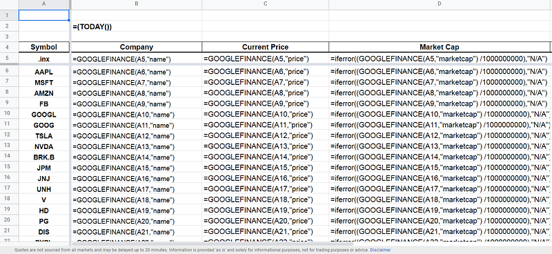
Cell B6 Formula: =GOOGLEFINANCE(A6,”name”)

Cell C6 Formula: =GOOGLEFINANCE(A6,”price”)

Cell D6 Formula: =iferror((GOOGLEFINANCE(A6,”marketcap”) /1000000000),”N/A”)

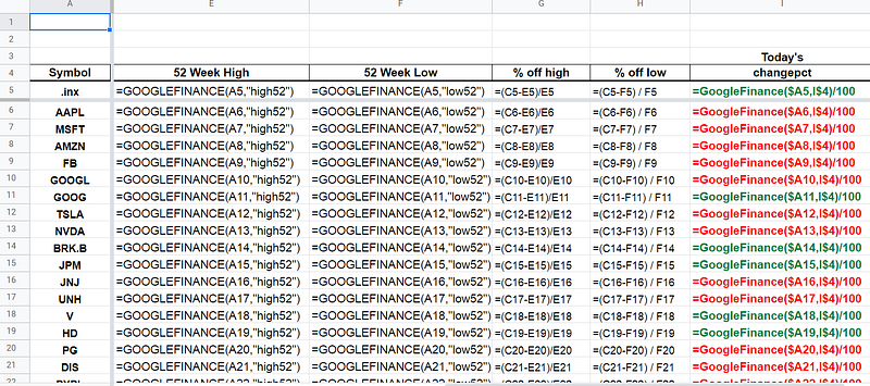
Cell E6: =GOOGLEFINANCE(A6,”high52")

Cell F6: =GOOGLEFINANCE(A6,”low52")

Cell G6: =(C6-E6)/E6

Cell H6: =(C6-F6) / F6

Any guesses on cell I6??

That was a trick question! This is the column that is different than all others and based on the changepct from the beginning.

Cell I6: =GoogleFinance($A6,I$4)/100

It is important to lock the I4, so when you drag it down, it stays in cell I4 and does not move.

Now just copy row 6 down to all the other rows.

You’re file should be looking really good by now.

(I included screenshots of the formulas at the end of the article in case those are easier to understand.)

Conditional Formatting

Eighty percent of data science is cleaning data and the other twenty percent is complaining about cleaning data

- Anthony Goldbloom

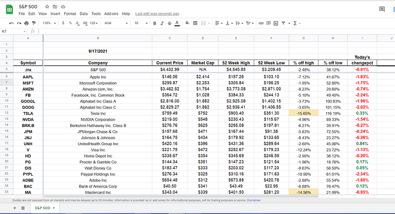
All this data is cool, but right now it's just a shit ton of numbers. It’s too much information to analyze. I applied conditional formatting to my data to better understand it.

There were two conditional formats — one for the changepct and one for %offhigh.

To create conditional formats, highlight the entire column, then go to Format -> Conditional Formatting -> then go to the format rules section.

For %offhigh, which is the main point of this file, format cells if less than or equal to…whatever number you want. I choose -.14 for this example. I will likely change it to -.20. Then in formatting style, select the color and if you want the text or cell background to change.

You can also add a filter, to help you sort the data. Highlight the row with the headers, go to Data -> Create a filter. Then you can sort any row however you please.

Why this is helpful

The whole reason for this file is to help you monitor stocks you are interested in. Now you can see how much a stock is off its high and if it is a good time to buy.

It’s hard to keep track of so many stocks. And most of the time you only see the daily change. Now you can see what’s really going on, with one stock or the whole market. 13% of the S&P 500 is more than 20% below its high!

Extra Tips

I added a date at the top of my file — it’s not needed but I like it. It’s a check. Whenever I open the file I know what the current date is and that the other formulas are also updated.

The formula to get the current date is: =(TODAY())

If you have any questions or issues with this guide, please reach out. I’m hoping this is helpful to someone and might consider doing more of these in the future.