How to Run Bootstrap Analysis in BigQuery

Make the most out of the little data you have, by grabbing your data by the bootstraps.

Obligatory pair of boots with straps | created via DALLE

Introduction

Imagine you’re trying to gauge the average height of all the trees in a vast forest. It’s impractical to measure each one, instead, you measure a small sample and use those measurements to estimate the average for the entire forest. Bootstrapping, in statistics, works on a similar principle.

This involves taking a small sample from your data and, through a method of repeated sampling, estimates statistics (like the mean, median or standard deviation) for your dataset. This technique allows you to make inferences about populations from small samples with greater confidence.

In this article, we will cover:

The basics of bootstrapping, what is it exactly?
How to achieve a bootstrapped sample in BigQuery
An experiment to understand how results change based on varying sample sizes, and how that relates to a known statistic
A stored procedure you can take away and use yourself

Bootstrapping Basics

At its core, bootstrapping involves randomly selecting a number of observations from a dataset, with replacement, to form what is known as a “bootstrap sample.”

Let’s simplify this concept using a scenario where you have a basket of 25 apples and you’re curious about the average weight of apples in a larger context, like a market.

The Grab and Note Technique

Start by diving into your basket to grab an apple at random, weigh it, and then, instead of setting it aside, you put it right back into your basket. This way, every time you reach in for an apple, every single one, including the one you just weighed, is fair game to be picked again.

Repeat

Now, you repeat the grab, weigh, and replace action the same amount of times as there are apples in your basket, so 25 times in this scenario. Because you’re putting apples back after weighing them, you might end up weighing the same apple multiple times or possibly not at all. It’s the luck of the draw.

After completing 25 grabs, you have your first bootstrap sample. This sample is essentially a snapshot of potential average weights based on the apples you’ve randomly selected. To build a robust understanding, this process is often replicated hundreds or thousands of times.

These thousands of bootstrap samples serve as the foundation for understanding the variability and reliability of statistical estimates derived from limited data. This method’s strength lies in its ability to provide insight into the distribution of a statistic without relying on traditional assumptions, which might not always be valid or verifiable.

How to Generate a Bootstrap Sample in BigQuery

BigQuery doesn’t have a method for easily generating bootstrap samples, so we need to get a bit creative. I’ll start by using a small dataset of 25 rows.

Later, we will tackle a larger dataset with various sample and bootstrap sizes!

For this example, I’ve created a random dataset that simulates the weights of apples.

SELECT
    apples AS Apple_ID,
    CAST(FLOOR((RAND() + RAND() + RAND() + RAND() + RAND() + RAND() + RAND() + RAND() + RAND() + RAND()) / 10 * 200 + 100) AS INT64) AS weight
FROM
    UNNEST(GENERATE_ARRAY(1, 25)) AS apples

Step 1

Generate an array of integers between 1 and 25 using GENERATE_ARRAY(1, 25). Each integer represents an apple.

Step 2

Unnest the generated array to create a row for each apple.

Step 3

Calculate the weight for each apple. I’ve achieved this by averaging ten calls to RAND(), which generates a random number between 0 and 1 then scaling to fit within the 100 to 300-gram range.

The 10 calls to RAND brings in the central limit theorem to help build a normal distribution.

Finally, the weight is rounded down to the nearest whole number using FLOOR and cast to an INT64 type.

These 25 apples average at 198.48 in weight, which we will compare against when we’ve generated our bootstrap samples.

Step 1: Setting Up

To start, we’ll declare and set some variables.

DECLARE BOOTSTRAP_SAMPLES, SAMPLE_SIZE INT64;

SET BOOTSTRAP_SAMPLES = 100;
SET SAMPLE_SIZE = (SELECT COUNT(*) FROM medium_examples.Apples_Demonstration);

BOOTSTRAP_SAMPLES: The number of bootstrap samples we want to generate. In this example, we'll create 100 samples.
SAMPLE_SIZE: The number of data points in our dataset. This will be obtained from the dataset itself, as your sample size for each bootstrap should equal the size of the data source you’re sampling from.

Step 2: Generating Bootstrap Samples

The core of our bootstrapping method involves creating a mapping that allows us to select data points multiple times (with replacement).

Creating a mapping table: We use two arrays generated in BigQuery to create a mapping between bootstrap samples and total dataset rows. This mapping will ensure that each sample can include any data point multiple times, enabling the “with replacement” aspect of bootstrapping.

WITH mapping AS (
  SELECT 
    bootstrap_index,
    CAST(FLOOR(RAND() * SAMPLE_SIZE) AS INT64) + 1 AS row_num
  FROM 
    UNNEST(GENERATE_ARRAY(1, BOOTSTRAP_SAMPLES)) AS bootstrap_index, 
    UNNEST(GENERATE_ARRAY(1, SAMPLE_SIZE))
)

Step 3: Analysing Bootstrapped Data

After establishing our mapping, we join with the original dataset to compute the average weight of apples in each bootstrap sample.

WITH bootstrapped_data AS (
  SELECT 
    bootstrap_index,
    ROUND(AVG(weight), 2) AS avg_weight
  FROM 
    mapping
  LEFT JOIN 
    (
      SELECT
        weight,
        ROW_NUMBER() OVER () AS row_num
      FROM
        medium_examples.Apples_Demonstration
    )
    USING(row_num)
  GROUP BY
    bootstrap_index
)

This calculates the average weight of apples for each of the 100 bootstrapped samples.

Step 4: Obtaining Final Results

Finally, we calculate the overall average weight, standard error, and 95% confidence intervals from our bootstrapped samples

SELECT
  ROUND(AVG(avg_weight) OVER (), 2) AS weight_avg,
  ROUND(STDDEV(avg_weight) OVER (), 2) AS standard_error_weight,
  ROUND(PERCENTILE_CONT(avg_weight, 0.025) OVER (), 2) AS weight_low_interval,
  ROUND(PERCENTILE_CONT(avg_weight, 0.975) OVER (), 2) AS weight_high_interval
FROM bootstrapped_data
LIMIT 1

This leaves us with some stats that tell us more about how much our apples might weigh on average and the expected range. Here’s the gist:

Average Weight: We’ve got an average apple weight of 198.63 units.
Standard Error: The standard error is like a reality check, telling us how confident we can be about our average weight. Ours is 3.3 units, which is pretty good! It means our average weight isn’t just a wild guess; it’s a reliable estimate. My general rule of thumb is to divide standard error by the average weight, and if the outcome is less than 5% it indicates a relatively precise estimate across our samples (1.66% here).
Confidence Interval: This is our “safety net,” ranging from 192.11 to 205.9 units. It’s a way of saying, “We’re 95% sure the real average weight of all apples falls within this range”.

Here is the full query.

##############################################################
################### VARIABLE DECLARATION #####################
##############################################################

DECLARE BOOTSTRAP_SAMPLES, SAMPLE_SIZE INT64;
DECLARE ACTUAL_AVG FLOAT64;

##############################################################
###################### VARIABLE SETTING ######################
##############################################################

SET BOOTSTRAP_SAMPLES = 100;
SET SAMPLE_SIZE = (SELECT count(*) FROM medium_examples.Apples_Demonstration);

##############################################################
################ BOOTSTRAP SAMPLE GENERATOR ##################
##############################################################

WITH mapping as (
SELECT 
    bootstrap_index,
    cast(floor(rand() * SAMPLE_SIZE) as int64) + 1 as row_num
FROM 
    unnest(generate_array(1, BOOTSTRAP_SAMPLES)) as bootstrap_index, 
    unnest(generate_array(1, SAMPLE_SIZE))
),

bootstrapped_data as (
select 
    bootstrap_index,
    count(*) as total_rows,
    round(avg(weight), 2) as weight_avg
from 
    mapping
join 
    (
    SELECT
        weight,
        row_number() over () as row_num
    FROM
        medium_examples.Apples_Demonstration
    )
    using(row_num)
group by
    bootstrap_index
)

SELECT
    round(avg(weight_avg) over (), 2) as overall_weight_avg,
    round(stddev(weight_avg) over (), 2) as standard_error_weight,
    round(percentile_cont(weight_avg, 0.025) over (), 2) AS weight_low_interval,
    round(percentile_cont(weight_avg, 0.975) over (), 2) AS weight_high_interval
FROM 
    bootstrapped_data
LIMIT 1

Generating a Lot of Apples

Let’s take this a step further.

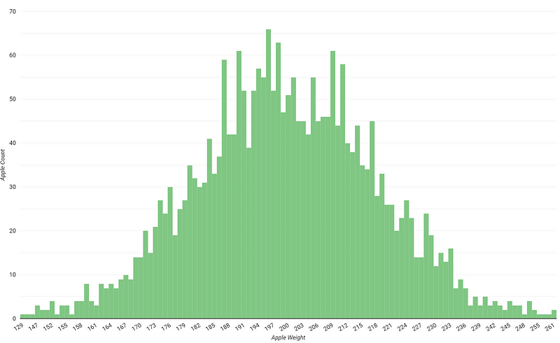
This time, I’m going to create a bunch of apples just like before, but we’re working with 2,500 apples this time, each weighing between 100 and 300 grams.

Imagine we’ve gone to a market and weighed every single apple there, so we can consider this dataset as our population which we will take samples from soon.

Checking the distribution in Looker Studio, we can see the dataset follows a nice bell-shaped curve as expected from our generator. This dataset has an average weight of 199.23.

Exploring Sample Sizes in Bootstrapping

When you’re dealing with real-world data, control over your sample size might not always be in your hands. You could be working with a fixed number of survey responses or volunteers for a study. Other times, you might choose your sample size without knowing the full extent of the population, like guessing the number of apples in a market or trees in a forest. Pinning down the total population can be challenging, if not outright impossible.

When bootstrapping, two frequently asked questions emerge:

How many bootstrap samples are ideal?
What’s the smallest sample size I can work with effectively?

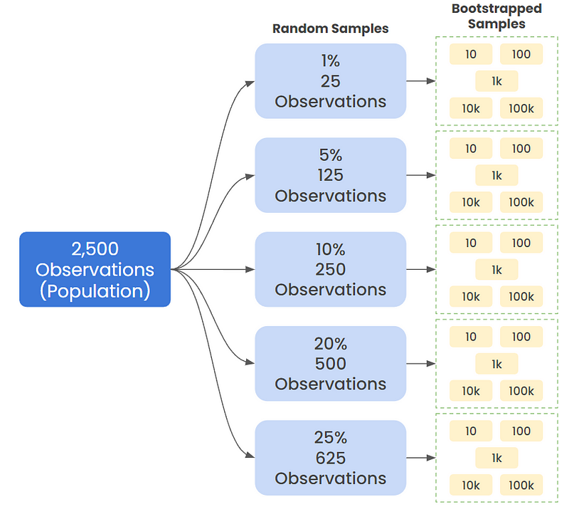
The truth is, there’s no one-size-fits-all answer. I plan to test a variety of sample sizes ranging from 1% to 25% of the population, with bootstrap sample sizes ranging from 10 to as many as 100,000.

This range will help examine how adjustments in size from small to large can shed light on the relationship between sample size, number of bootstrap samples, and the overall quality of our analysis.

The Results

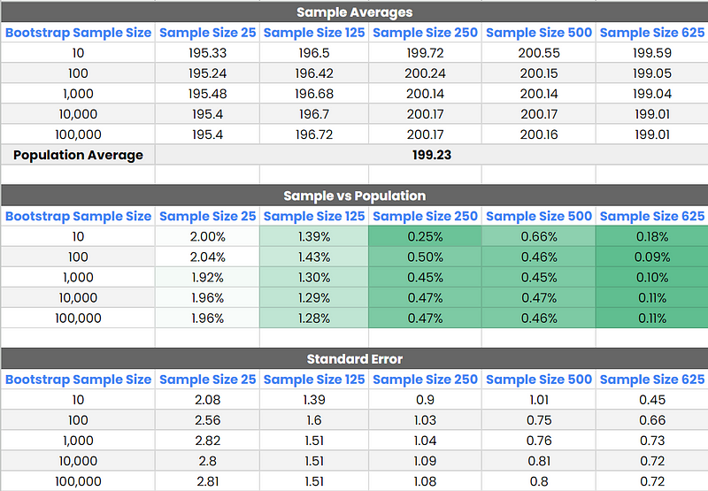
Comparing the bootstrap analysis outcomes with the actual population average of 199.23, we can draw several insights regarding the accuracy of each test and deduce the impact of varying sample sizes.

Key Points

Initial Variability: With 10 bootstrap samples, there’s a notable variance from the actual average across all sample sizes, indicating insufficient sampling.

Diminishing Returns Beyond 1,000 Bootstrap Samples: From 1,000 bootstrap samples onwards, changes in estimates become negligible. The results stabilize, suggesting that increasing the number of bootstrap samples beyond this point does little to improve accuracy.

Sample Size 500 and 625 — High Accuracy: Both demonstrated high accuracy, particularly from 100 bootstrap samples onward, closely mirroring the actual average, although these required a sample size of 20% and 25% of the population (respectively) which isn’t always achiveable.

From what I’ve found in my tests, taking a 10% chunk of our apple bunch (250 apples) and running 1,000 bootstrap samples hit the sweet spot. When I tried using more samples than that, the numbers didn’t really change much — they stayed pretty much in the same ballpark. This provides us with a 95% confidence interval of 198.03–202.13.

The Query

Admittedly, I might have gone a bit overboard with my approach this time, driven by the thrill of tackling a challenge. Instead of manually adjusting and executing the bootstrap generator for each of the 25 scenarios shown earlier, I crafted a single query that autonomously manages the entire process.

In case you’re interested, I’ve included my query below.

##############################################################
################### VARIABLE DECLARATION #####################
##############################################################

DECLARE DESTINATION_TABLE, TARGET_TABLE, REGION, TABLE_ID, METRIC, QUERY STRING;
DECLARE TEMP_TABLES ARRAY<STRING>;
DECLARE SAMPLE_SIZE, BOOTSTRAP_SAMPLE, TABLE_ROWS INT64;
DECLARE LOOP_COUNTER, LOOP_COUNTER_INNER INT64 DEFAULT 1;
DECLARE BOOTSTRAP_SAMPLES, TOTAL_ROWS ARRAY<INT64>;
DECLARE PERC_OF_SAMPLE ARRAY<FLOAT64>;

##############################################################
###################### VARIABLE SETTING ######################
##############################################################

SET TARGET_TABLE = 'spreadsheep-20220603.medium_examples.Apples';
SET BOOTSTRAP_SAMPLES = [10, 100, 1000, 10000, 100000];
SET REGION = 'region-US';
SET PERC_OF_SAMPLE = [0.01, 0.05, 0.1, 0.2, 0.25];
SET METRIC = 'weight';

EXECUTE IMMEDIATE ("select total_rows from "||REGION||".INFORMATION_SCHEMA.TABLE_STORAGE_BY_PROJECT where table_schema = split('"||TARGET_TABLE||"', '.')[1] and table_name = split('"||TARGET_TABLE||"', '.')[2]") INTO SAMPLE_SIZE;

##############################################################
#################### TEMP TABLES CREATION ####################
##############################################################

REPEAT

    SET TABLE_ID = split(TARGET_TABLE, '.')[2]||"_"||CAST(PERC_OF_SAMPLE[ORDINAL(LOOP_COUNTER)] * 100 AS INT64)||"_perc_sample";
    SET TEMP_TABLES = IF(TEMP_TABLES IS NULL, [TABLE_ID], ARRAY_CONCAT(TEMP_TABLES, [TABLE_ID]));

    SET TABLE_ROWS = CAST(SAMPLE_SIZE * PERC_OF_SAMPLE[ORDINAL(LOOP_COUNTER)] AS INT64);
    SET TOTAL_ROWS = IF(TOTAL_ROWS IS NULL, [TABLE_ROWS], ARRAY_CONCAT(TOTAL_ROWS, [TABLE_ROWS]));

    EXECUTE IMMEDIATE ("CREATE TEMP TABLE `"||TABLE_ID||"` AS (SELECT * FROM "||TARGET_TABLE||" ORDER BY RAND() LIMIT "||TABLE_ROWS||")");
    
    SET LOOP_COUNTER = LOOP_COUNTER + 1;
    UNTIL LOOP_COUNTER > ARRAY_LENGTH(PERC_OF_SAMPLE)

END REPEAT;

##############################################################
################ BOOTSTRAP SAMPLE GENERATOR ##################
##############################################################

SET LOOP_COUNTER = 1;

REPEAT
    SET TABLE_ID = TEMP_TABLES[ORDINAL(LOOP_COUNTER)];

    REPEAT
        SET BOOTSTRAP_SAMPLE = BOOTSTRAP_SAMPLES[ORDINAL(LOOP_COUNTER_INNER)];


        CREATE OR REPLACE TEMP TABLE bootstrap_selection_generator as (
        select 
            bootstrap_index,
            cast(floor(rand() * TOTAL_ROWS[ORDINAL(LOOP_COUNTER)]) as int64) as row_num
        from 
            unnest(generate_array(1, BOOTSTRAP_SAMPLE)) as bootstrap_index, 
            unnest(generate_array(1, TOTAL_ROWS[ORDINAL(LOOP_COUNTER)]))
        );

        SET QUERY = CONCAT(
            "select "||TOTAL_ROWS[ORDINAL(LOOP_COUNTER)]||", concat('sample_"||BOOTSTRAP_SAMPLE||"','_',bootstrap_index), avg("||METRIC||") from bootstrap_selection_generator ",
            "left join (SELECT "||METRIC||", row_number() over () as row_num FROM "||TABLE_ID||") using(row_num) group by 1,2");

        EXECUTE IMMEDIATE ("insert into spreadsheep-20220603.medium_examples.Apple_Samples ("||QUERY||")");

        SET LOOP_COUNTER_INNER = LOOP_COUNTER_INNER + 1;
        UNTIL LOOP_COUNTER_INNER > ARRAY_LENGTH(BOOTSTRAP_SAMPLES)
    END REPEAT;

    SET LOOP_COUNTER_INNER = 1;

    SET LOOP_COUNTER = LOOP_COUNTER + 1;
    UNTIL LOOP_COUNTER > ARRAY_LENGTH(TEMP_TABLES)
END REPEAT

Random Distribution

In previous section, we worked with data that fit a nice, bell-shaped curve. Now, I’m curious about what happens when we use a completely random distribution instead.

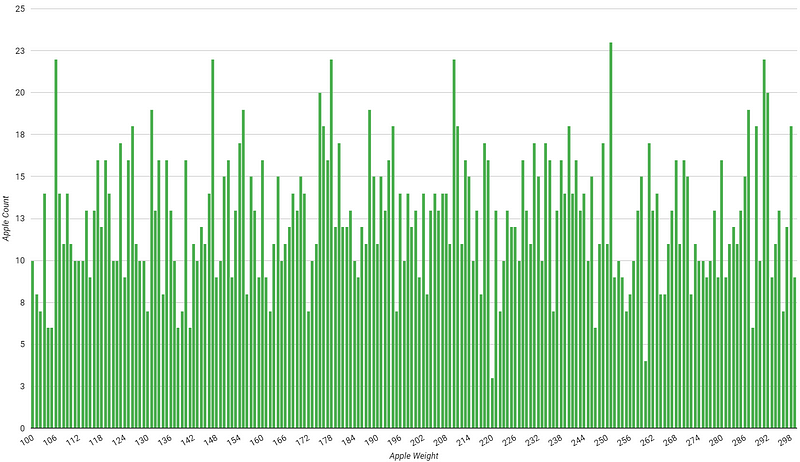
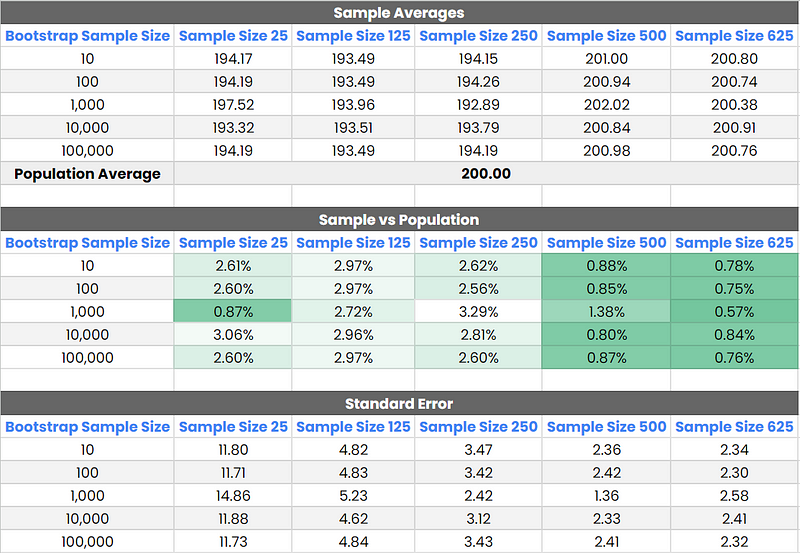
My findings suggest that hitting the population average with a random distribution is a bit tougher. However, the pattern regarding the optimal bootstrap sample size still holds. Starting with 1,000 bootstrap samples proves effective, particularly when using a 20% sample size of our data. For this scenario, the 95% confidence interval stretched from 196.41 to 205.80, nicely encompassing the true average of 200.00.

Standard error rates were on the higher side for smaller sample sizes. This hints that leaning towards a larger sample size might be a smart move when dealing with data that shows more unpredictability.

Bootstrap Stored Procedure

To make my bootstrap analyses easier down the line, I’ve created a stored procedure. This is designed so that both I and my team members can run our analyses more smoothly in the future.

Here’s all you need to do to use it:

Bootstrap Samples: Decide how many bootstrap samples you’d like to generate.
Sample Size: Choose your sample size, which should match the total number of rows in your table.
Table ID: Identify the table_id of the table you’re bootstrapping from.
Metric: Select the metric you’re aiming to measure.

CREATE OR REPLACE PROCEDURE `spreadsheep-20220603.medium_examples.bootstrap_generator`(BOOTSTRAP_SAMPLES INT64, SAMPLE_SIZE INT64, TABLE_ID STRING, METRIC STRING)
BEGIN

DECLARE QUERY STRING;

SET QUERY = CONCAT("with mapping as (select bootstrap_index, cast(floor(rand() * "||SAMPLE_SIZE||") as int64) + 1 as row_num ",
                   "from unnest(generate_array(1, "||BOOTSTRAP_SAMPLES||")) as bootstrap_index, unnest(generate_array(1, "||SAMPLE_SIZE||"))), \n\n");

SET QUERY = CONCAT(QUERY, "bootstrapped_data as (select bootstrap_index, round(avg("||METRIC||"), 2) as metric from mapping ",
                          "left join (SELECT "||METRIC||", row_number() over () as row_num FROM "||TABLE_ID||") using(row_num) group by bootstrap_index) \n\n");

SET QUERY = CONCAT(QUERY, "SELECT avg(metric) over () as bootstrap_average, stddev(metric) over () as standard_error, ",
                          "percentile_cont(metric, 0.025) over () AS confidence_interval_lower_bound, percentile_cont(metric, 0.975) over () AS confidence_interval_upper_bound FROM bootstrapped_data LIMIT 1");
                          
SELECT QUERY;
EXECUTE IMMEDIATE(QUERY);
END

That brings this article to an end. If you have any questions or challenges, please feel free to comment, and I’ll answer when I can.

I frequently write articles for BigQuery and Looker Studio. If you’re interested, consider following me here on Medium for more!

All images, unless otherwise noted, are by the author.

Stay classy folks! Tom

Summarize