
How to Remove Non-Stationarity in Time Series Forecasting
Algorithms can’t handle non-stationary. They need static relationships.

Introduction
Unlike ordinary machine learning problems, time series forecasting requires extra preprocessing steps.
On top of the normality assumptions, most ML algorithms expect a static relationship between the input features and the output.
A static relationship requires inputs and outputs with constant parameters such as mean, median, and variance. In other words, algorithms perform best when the inputs and outputs are stationary.
This is not the case in time series forecasting. Distributions that change over time can have unique properties such as seasonality and trend. These, in turn, cause the mean and variance of the series to fluctuate, making it hard to model their behavior.
So, making a distribution stationary is a strict requirement in time series forecasting. In this article, we will explore several techniques to detect non-stationary distributions and convert them into stationary data.
You can access all the articles in this Time Series Forecasting series from here.
Get the best and latest ML and AI papers chosen and summarized by a powerful AI — Alpha Signal:
Why is stationarity important?
If a distribution is not stationary, then it becomes tough to model. Algorithms build relationships between inputs and outputs by estimating the core parameters of the underlying distributions.
When these parameters are all time-dependent, algorithms will face different values at each point in time. And if the time series is granular enough (such as minutes or seconds frequencies), models may even end up with more parameters than actual data.
This type of variable relationship between inputs and outputs will seriously compromise the decision function of any model. If the relationship keeps changing through time, models end up using an outdated relationship or one that does not contribute to its predictive power.
Therefore, you must dedicate a certain amount of time to detecting non-stationarity and removing its effects during your workflow.
We will see an example of this in the coming sections.
Examples of non-stationary series
Take a look at these plots and try to guess which of the lines represent a stationary series:
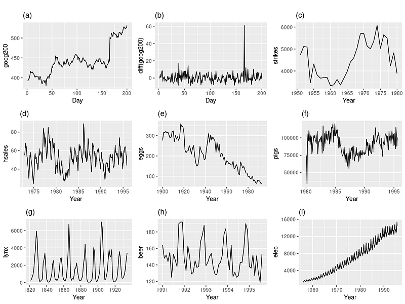
Since stationary series have constant variance, we can rule out a, c, e, f, and i. These plots show a clear upward or downward trend or changing levels like in f.
Similarly, as d and h show seasonal patterns, we can rule them out too.
But how about g — the pattern does look it is seasonal.
g is the plot of the lynx population growth. When food becomes scarce, they stop breeding, causing the population numbers to plummet. When the food sources replenish, they start reproducing again, making the population grow.
This cyclic behavior is not the same as seasonality. When seasonality exists, you know exactly what will happen after a certain period of time. In contrast, the cyclic behavior of lynx population growth is unpredictable. You can’t guess the timing of the food cycles and this makes the series stationary.
So, the only stationary series are b and g.
Tricky distributions like d, f, and h can make you question whether identifying non-stationary data visually is the best option. As you observed, it is pretty easy to confuse seasonality with random cycles or trends with white noise.
For this reason, the next section will be about statistical methods of detecting non-stationary time series.
Detecting non-stationarity statistically
In the statistics world, there are several tests under the label of unit root tests. The augmented Dickey-Fuller test may be the most popular one, and we have already seen how to use it to detect random walks in my last post.
Here, we will see how to use it to check if a series is stationary or not.
Simply put, here are the null and alternative hypotheses of this test:
- The null hypothesis: the distribution is non-stationary, time-dependent (it has a unit root).
- The alternative hypothesis: the distribution is stationary, not time-dependent (can’t be represented by a unit root).
The p-value determines the result of the test. If it is smaller than a critical threshold of 0.05 or 0.01, we reject the null hypothesis and conclude that the series is stationary. Otherwise, we fail to reject the null and conclude the series is non-stationary.
The full test is conveniently implemented as adfuller function under statsmodels. First, let's use it on a distribution we know is stationary and get familiarized with its output:
We look at the p-value, which is almost 0. This means we can easily reject the null and consider the distribution as stationary.
Now, let’s load the TPS July Playground dataset from Kaggle and check if the target carbon monoxide is stationary:
Surprisingly, carbon monoxide is found to be stationary. This might be because the data is recorded over a short period of time, which diminishes the effect of the time component. In fact, all other variables in the data are completely stationary.
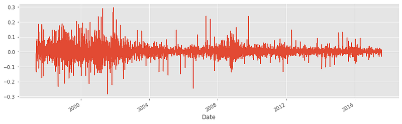
Now, let’s load some financial data that is more likely to be non-stationary:
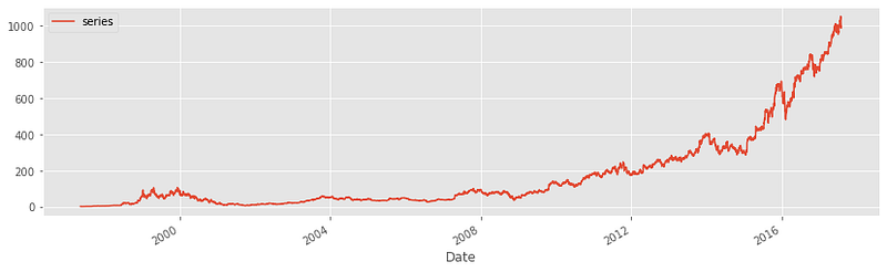
Some of the datasets have been anonymized due to publication policies. But you can check out the Kaggle notebook here for the original version. Note that this anonymity won’t hinder your understanding of the content.
As you can see, the series shows a clear upward trend. Let’s perform the Dickey-Fuller test:
We get a perfect p-value of 1 — this is 100% non-stationary time series data. Let’s perform a final test on another distribution, and we will move on to different techniques you can deal with this type of data:
The p-value is close to 1. No interpretation is necessary.
Transforming non-stationary series to make it stationary
One method for transforming the simplest non-stationary data is differencing. This process involves taking the differences of consecutive observations. Pandas has a diff function to do this:
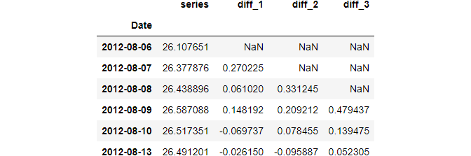
The output above shows the results of first, second, and third-order differencing.
For simple distributions, taking the first-order difference is enough to make it stationary. Let’s check this by using the adfuller function on the diff_1 (first-order difference of ts2):
When we run adfuller on the original distribution ts2, the p-value was close to 1. After differencing, the p-value is flat 0, suggesting we reject the null and conclude the series is now stationary.
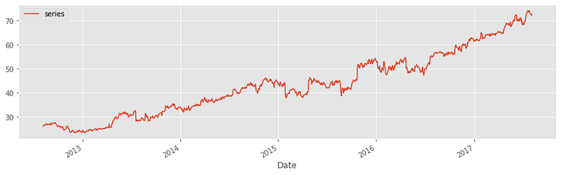
However, some distributions may not be so easy to deal with. Consider this one we saw earlier:
Before taking the difference, we have to account for that obvious non-linear trend. Otherwise, the series will still be non-stationary.
To remove non-linearity, we will use the logarithmic function np.log and then, take the first-order difference:
As you can see, the distribution that returned a perfect p-value before transformation is now completely stationary.
Below is the plot of monthly antibiotics sales in Australia:
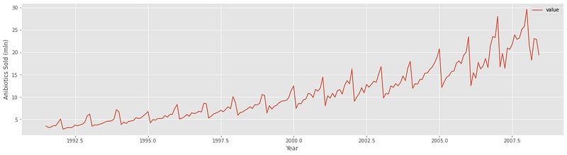
As you can see, the series shows both an upward trend and a strong seasonality. We will again apply a log transform and, this time, take a yearly difference (365 days or 12 months) to remove the seasonality.
Here is what each step looks like:
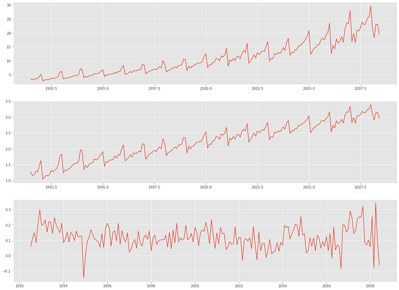
We can confirm the stationarity with adfuller:
The p-value is extremely small, proving that the transformation steps have shown their effect.
In general, every distribution is different, and to achieve stationarity, you might end up changing multiple operations. Most of these involve taking logarithms, first/second-order, or seasonal differencing.
Summary
Another topic is done and dusted in this Time Series forecasting series!
We have already covered a lot, even though we haven’t gotten around to the actual forecasting part. By now, you should be able to:
- Manipulate time-series data like a pro using pandas (link).
- Dissect any time series into core components such as seasonality and trend (link).
- Analyze time-series signals using autocorrelation (link).
- Identify if the target you want to predict is white noise or follows a random walk (link).
And finally, you learned how to remove the effect of non-stationary from any time series. All of these are must-know topics and important building blocks to forecasting. The next post is on time-series feature engineering. Don’t miss it!
Loved this article and, let’s face it, its bizarre writing style? Imagine having access to dozens more just like it, all written by a brilliant, charming, witty author (that’s me, by the way :).
For only 4.99$ membership, you will get access to not just my stories, but a treasure trove of knowledge from the best and brightest minds on Medium. And if you use my referral link, you will earn my supernova of gratitude and a virtual high-five for supporting my work.


