How to Optimize Hyperparameters for Machine Learning Models

With video explanation | Data Series | Episode 12.1

This article looks at the various methods used to optimise hyperparameters for a machine learning model. These are:

1. Manual Search
2. Grid Search
3. Random Search
4. Bayesian Optimization

We also look at

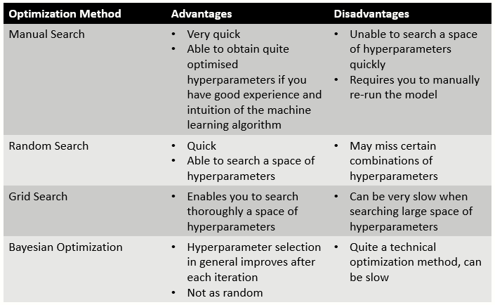
5. Advantages and Disadvantages of Optimization Methods

Before looking into these methods it is important we have a good understanding of what hyperparameters are:

What are Hyperparameters?

A parameter is what the machine learning algorithm learns. For example, we may choose a model of the form:

After training the model using gradient descent:

We obtain θ₀ = 1.5 and θ₁ = 2. θ₀ and θ₁ are parameters learnt from gradient descent and therefore are just regular parameters.

Hyperparameters are the parameters used to control the learning process and structure of the model. In the above example to find the values of θ₀ and θ₁ we are required to set the learning rate α for gradient descent. α here is a hyperparameter.

The parameters that we set in a model are often hyperparameters. For example in gradient boosted trees — the number of trees and depth of the trees are considered hyperparameters as we can set these ourselves.

Manual Search

Manual search relies on past experience and intuition of machine learning algorithms to set hyperparameters. For example with gradient boosted trees on large complex datasets we know we may need a lot of trees and a small learning rate alpha. We would try this to start with and adjust according to the model’s performance.

For smaller dataset, we would look at having a smaller number of trees and perhaps lower tree depth.

Random Search

For random search we define a space of hyperparameters to randomly sample from. For example:

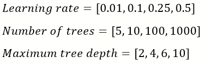
We then randomly sample from this space. Here we choose 5 samples.

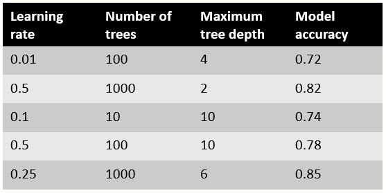
We then select the hyperparameter combination that leads to the best model performance which in example above is a learning rate of 0.25, number of trees of 1000 and maximum tree depth of 6.

Grid Search

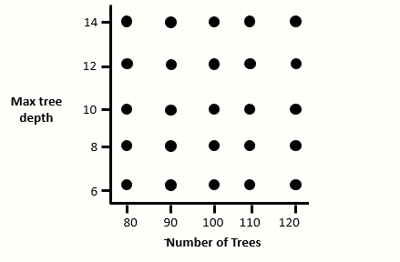
Grid search, also known as parameter sweep searches manually through a set of hyperparameters. For example, if we wanted to optimise the number and depth of trees of a gradient boosting algorithm we would make the following grid:

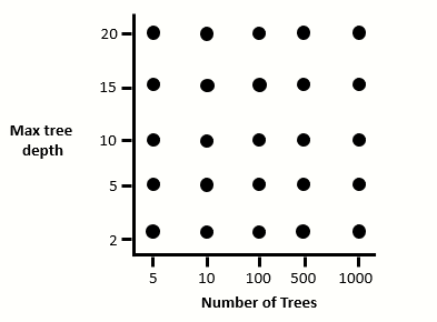
The grid search algorithm would then try every combination of hyperparamater: 5 trees at 2 depth, 5 trees at 5 depth, 5 trees at 10 depth and so on….. and evaluate these combinations on a validation set of data.

After finding the hyperparameters that lead to the best model performance on the validation set, let us say for example it is 100 trees at a depth of 10, we could then narrow the grid search further:

We can keep doing this until we are satisfied with the model’s performance.

Bayesian Optimization

Bayesian optimization works by trying to estimate a function that shows the relationship between our target value and the model’s hyperparameters.

For example, let us say we were looking at accuracy as out target value and we wanted to optimise the learning rate alpha. The function that Bayesian optimization is trying to estimate and find the maximum of is:

For machine learning algorithms with many parameters we would be looking to estimate a multi-dimensional function.

Note: The above function is not known — bayesian optimization tries to estimate and find the maximum of this.

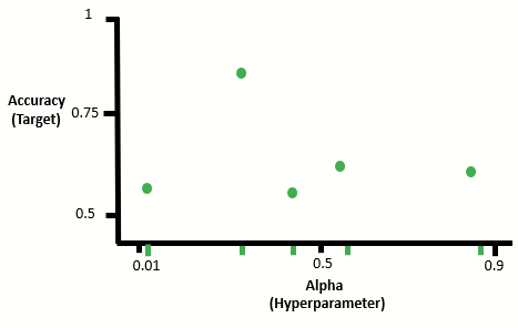
1. First we start by producing sample values of alpha and calculate the resulting accuracy. There are many ways to produce these sample values, here we focus on random sampling — where we randomly select alpha values to test:

2. We then train a Gaussian regressor on the sampled values to estimate the function from these sampled points:

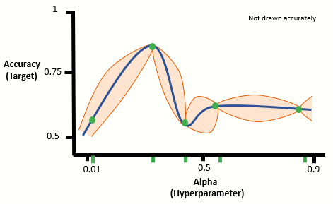
Here we train many regression functions and calculate the mean regression function indicated by the solid blue line. The orange area gives the uncertainty of of our model.

3. We then calculate what is called an Acquisition function that indicates to us the potential gain of searching an area. We check which point gives us the most gain and add this:

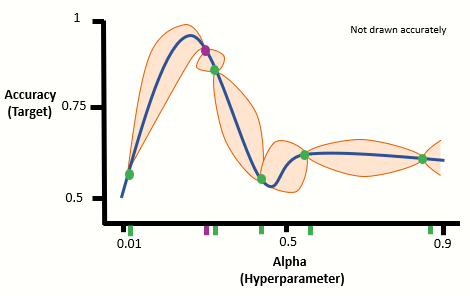
4. We repeat step 3 until for a set number of iterations. Lets us add two more iterations:

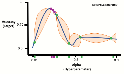
From our Bayesian Optimization algorithm, after 3 iterations, we find the optimal alpha value to be around 0.25.

Advantages and Disadvantages of Optimization Methods

Prev Episode | Next Episode

If you have any questions please leave them below!