Getting Started

How to Master Scikit-learn for Data Science

Here’s the Essential Scikit-learn you Need for Data Science

Scikit-learn is one of many scikits (i.e. short form for SciPy Toolkits) that specializes on machine learning. A scikit represents a package that is too specialized to be included in SciPy and are thus packaged as one of many scikits. Another popular scikit is the scikit-image (i.e. collection of algorithms for image processing).

Scikit-learn is by far one of the pillars for machine learning in Python as it allows you to build machine learning models as well as providing utility functions for data preparation, post-model analysis and evaluation.

In this article, we will be exploring the essential bare minimal knowledge that you need in order to master scikit-learn for getting started in data science. I try my best to distill the essence of the scikit-learn library through the use of hand-drawn illustrations of key concepts as well as code snippets that you can use for your own projects.

Let’s dive in!

1. Data representation in scikit-learn

Let’s start with the basics and consider the data representation used in scikit-learn, which is essentially a tabular dataset.

At a high-level, for a supervised learning problem the tabular dataset will be comprised of both X and y variables while an unsupervised learning problem will constitute of only X variables.

At a high-level, X variables are also known as independent variables and they can be either quantitative or qualitative descriptions of samples of interests while the y variable is also known as the dependent variable and they are essentially the target or response variable that predictive models are built to predict.

A cartoon illustration of a typical tabular data that is used in scikit-learn is shown below.

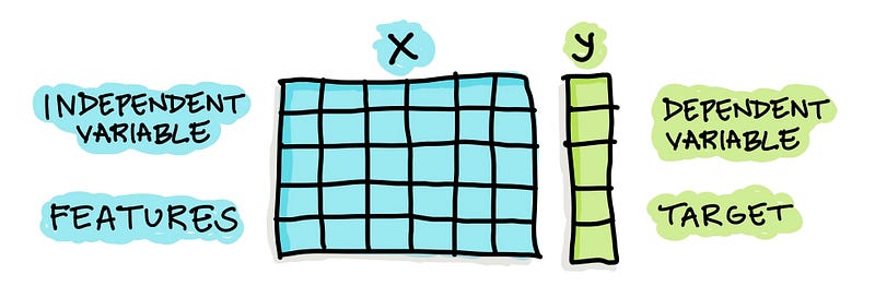
For example, if we’re building a predictive model to predict whether individuals have a disease or not the disease/non-disease status is the y variable whereas health indicators obtained by clinical test results are used as X variables.

2. Loading data from CSV files via Pandas

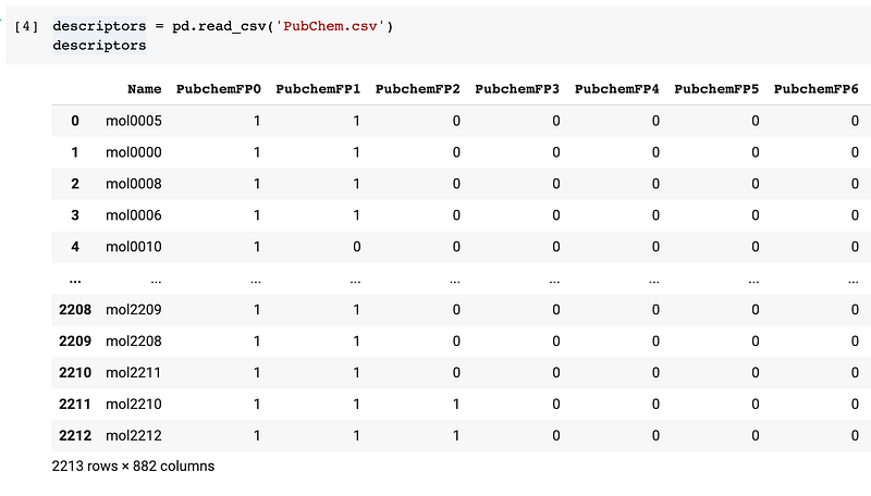
Practically, the contents of a dataset can be stored in a CSV file and it can be read in using the Pandas library via the pd.read_csv() function. Thus, the data structure of the loaded data is known as the Pandas DataFrame.

Let’s see this in action.

Afterwards, data processing can be performed on the DataFrame using the wide range of Pandas functions for handling missing data (i.e. dropping missing data or filling them in with imputed values), selecting specific column or range of columns, performing feature transformations, conditional filtering of data, etc.

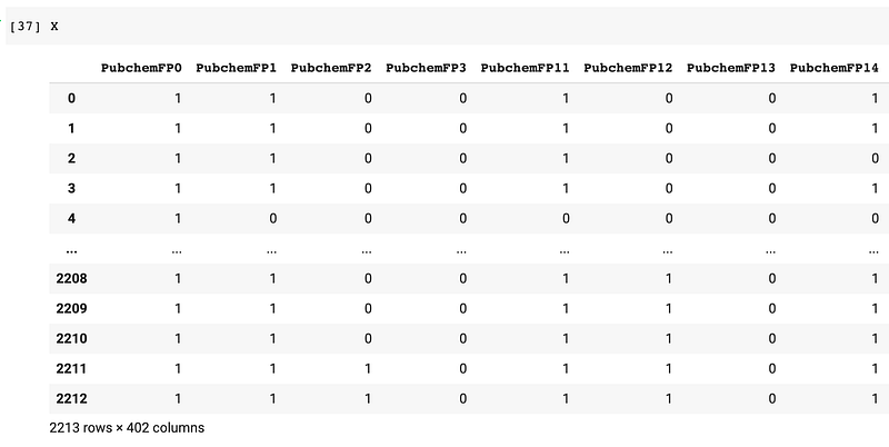
In the following example, we will separate the DataFrame as X and y variables, which will be used shortly for model building.

This gives rise to the following X data matrix:

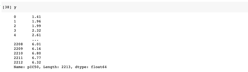
And the following y variable:

For a high-level overview of how to master Pandas for data science also check out a prior blog post that I’ve written.

3. Utility functions from scikit-learn

One of the great things about scikit-learn aside from its machine learning capability is its utility functions.

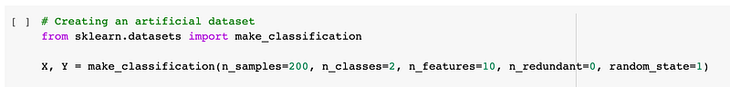
3.1. Creating artificial datasets

For instance, you can create artificial datasets using scikit-learn (as shown below) that can be used to try out different machine learning workflow that you may have devised.

3.2. Feature scaling

As features may be of heterogeneous scales with several magnitude difference, it is therefore essential to perform feature scaling.

Common approaches include normalization (scaling features to a uniform range of 0 and 1) and standardization (scaling features such that they have centered mean and unit variance that is all X features will have a mean of 0 and standard deviation of 1).

In scikit-learn, normalization can be performing using the normalize() function while standardization can be performed via the StandardScaler() function.

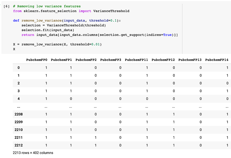
3.3. Feature selection

A common feature selection approach that I like to use is to simply discard features that have low variance as they provide minimal signal (if we think of it in terms of signals and noises).

3.4. Feature engineering

It is often the case that provided features may not readily be suitable for model building. For instance, categorical features require us to encode such features to a form that is compatible with machine learning algorithms in scikit-learn (i.e. from strings to integers or binary numerical form).

Two common types of categorical features includes:

1. Nominal features — Categorical values of the feature has no logical order and are independent from one another. For instance, categorical values pertaining to cities such as Los Angeles, Irvine and Bangkok are nominal.
2. Ordinal features — Categorical valeus of the feature has a logical order and are related to one another. For instance, categorical values that follow a scale such as low, medium and high has a logical order and relationship such that low < medium < high.

Such feature encoding can be performed using native Python (numerical mapping), Pandas (get_dummies() function and map() method) as well as from within scikit-learn (OneHotEncoder(), OrdinalEncoder(), LabelBinarizer(), LabelEncoder(), etc.).

3.5. Imputing missing data

Scikit-learn also supports the imputation of missing values, which is an important part of data pre-processing prior to the construction of machine learning models. Users can use either the univariate or multivariate imputation method via the SimpleImputer() and IterativeImputer() functions from the sklearn.impute sub-module.

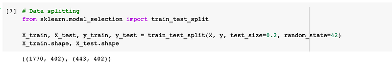
3.6. Data splitting

A commonly used function would have to be data splitting for which we can separate the given input X and y variables as training and test subsets (X_train, y_train, X_test and y_test).

The code snippet below makes use of the train_test_split() to perform the data splitting where its input arguments are the input X and y variables, the size of the test set set to 0.2 (or 20%) and a random seed number set to 42 (such that the code block will yield the same data split if it is ran multiple times).

3.7. Creating a workflow using Pipeline

As the name implies, we can make use of the Pipeline() function to create a chain or sequence of tasks that are involved in the construction of machine learning models. For example, this could be a sequence that consists of feature imputation, feature encoding and model training.

We can think of pipelines as the use of a collection of modular Lego-like building blocks for building machine learning workflows.

For more information on building your own machine learning pipeline using scikit-learn, Jason Brownlee from Machine Learning Mastery provides a detailed account in the following tutorial:

4. High-level overview of using scikit-learn

4.1. Core steps for building and evaluating models

In a nutshell, if I can summarize the core essence of using learning algorithms in scikit-learn it would consist of the following 5 steps:

from sklearn.modulename import EstimatorName      # 0. Import
model = EstimatorName()                           # 1. Instantiate
model.fit(X_train, y_train)                       # 2. Fit
model.predict(X_test)                             # 3. Predict
model.score(X_test, y_test)                       # 4. Score

Translating the above pseudo-code to the construction of an actual model (e.g. classification model) by using the random forest algorithm as an example would yield the following code block:

from sklearn.ensemble import RandomForestClassifier
rf = RandomForestClassifier(max_features=5, n_estimators=100)
rf.fit(X_train, y_train)
rf.predict(X_test)
rf.score(X_test, y_test)

A cartoon illustration summarizing these core basic steps for using estimators (i.e. the learning algorithm function) in scikit-learn is shown below.

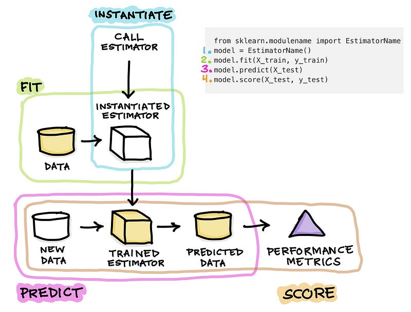
Step 0. Importing the estimator function from a module of scikit-learn. An estimator is used to refer to the learning algorithm such as RandomForestClassifier that is used to estimate the output y values given the input X values.

Simply put, this can be best summarized by the equation y = f(X) where y can be estimated given known values of X.

Step 1. Instantiating the estimator or model. This is done by calling the estimator function and simply assigning it to a variable. Particularly, we can name this variable as model, clf or rf (i.e. abbreviation of the learning algorithm used, random forest).

The instantiated model can be thought of as an empty box with no trained knowledge from the data as no training has yet occured.

Step 2. The instantiated model will now be allowed to learn from a training dataset in a process known as model building or model training.

The training is initiated via the use of the fit() function where the training data is specified as the input argument of the fit() function as in rf.fit(X_train), which literally translates to allowing the instantiated rf estimator to learn from the X_train data. Upon completion of the calculation, the model is now trained on the training set.

Step 3. The trained model will now be applied to make predictions on a new and unseen data (e.g. X_test) via the use of the predict() function.

As a result, predicted y values (y_test) are generated (and can be stored into a variable such as y_test_pred that can later be used for computing the model performance).

Step 4. The model performance can now be calculated. The simplest and quickest method is to use the score() function as in model.score(X_test, y_test).

If this function is used for a classification model the score() function produces the accuracy value whereas if it is a regression model the score() function calculates the R2 value.

For completeness, we can then extend this core workflow to also include other additional steps that could further boost the robustness and usability of constructed models.

I’ll be talking about these additional steps separately in the following sections.

4.2. Model interpretation

A model is only useful if insights can be extracted from it so as to drive the decision-making process.

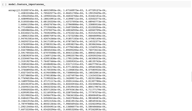
In continuation of the random forest model built above, important features stored in the instantiated rf model can be extracted as follows:

# Model interpretation

rf.feature_importances_

The above code would produces the following an array of importance values for features used in model building:

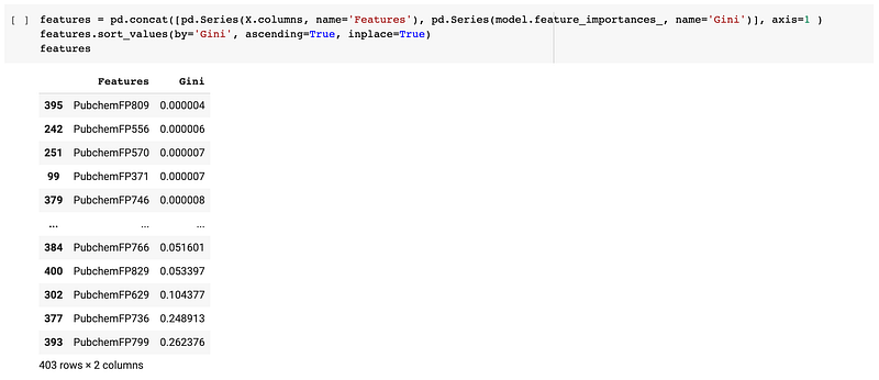
We can then tidy up the representation by combining it with the feature names to produce a clean DataFrame as follows:

Finally, one can take these values to create a feature importance plot as shown below:

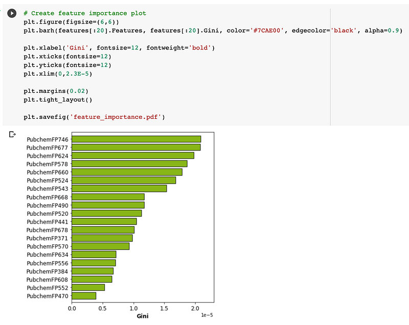
In a nutshell, as the name implies a feature importance plot provides the relative importance of features as judged by importance value such as those obtained from Gini indices produced by the random forest model.

4.3. Hyperparameter tuning

Typically, I would use default hyperparameters when building the first few models. At the first few attempts the goal is to make sure that entire workflow works synchronously and does not spit out errors.

My go-to machine learning algorithm is random forest and I use it as the baseline model. In many cases it is also selected as the final learning algorithm as it provides a good hybrid between robust performance and excellent model interpretability.

Once the workflow is in place, the next goal is to perform hyperparameter tuning in order to achieve the best possible performance.

Although random forest may work quite good straight out of the box but with some hyperparameter tuning it could achieve slightly higher performance. As for learning algorithms such as support vector machine, it is essential to perform hyperparameter tuning in order to obtain robust performance.

Let’s now perform hyperparameter tuning which we can perform via the use of the GridSearchCV() function.

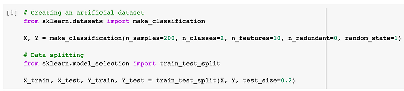
1. Firstly, we will create an artificial dataset and perform data splitting, which will then serve as the data for which to build subsequent models.

2. Secondly, we will now perform the actual hyperparameter tuning

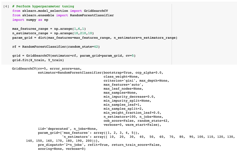
3. Finally, we can display the results from hyperparameter tuning in a visual representation.

You can download the full Jupyter notebook from which the above code snippets was taken from. If video is your thing, I’ve also created a YouTube video showing how to perform hyperparameter tuning using scikit-learn.

5. Example machine learning workflow

In this section, I will provide an example workflow that you can use as a general guideline that can be adapted to your own projects. Feel free to experiment with and tweak the procedures mentioned herein.

The first 6 steps can be performed using Pandas whereas subsequent steps are performed using scikit-learn, Pandas (to display results in a DataFrame) and also matplotlib (for displaying plots of model performance or plots of feature importance).

1. Read in the data as a Pandas DataFrame and display the first and last few rows.
2. Display the dataset dimension (how many rows and columns).
3. Display the data types of the columns and summarize how many columns are categorical and numerical data types.
4. Handle missing data. First check if there are missing data or not. If there are, make a decision to either drop the missing data or to fill the missing data. Also, be prepared to provide a reason justifying your decision.
5. Perform Exploratory data analysis. Use Pandas groupby function (on categorical variables) together with the aggregate function as well as creating plots to explore the data.
6. Assign independent variables to the X variable while assigning the dependent variable to the y variable
7. Perform data splitting (using scikit-learn) to separate it as the training set and the testing set by using the 80/20 split ratio (remember to set the random seed number).
8. Use the training set to build a machine learning model using the Random forest algorithm (using scikit-learn).
9. Perform hyperparameter tuning coupled with cross-validation via the use of the GridSearchCV() function.
10. Apply the trained model to make predictions on the test set via the predict() function.
11. Explain the obtained model performance metrics as a summary Table with the help of Pandas (I like to display the consolidated model performance as a DataFrame) or also display it as a visualization with the help of matplotlib.
12. Explain important features as identified by the Random forest model.

6. Resources for Scikit-learn

All aspiring and data science practitioners would typically find it necessary to once in a while take a glance at the API documentation or even cheat sheets to quickly find the precise functions or input arguments for the myriad of functions available from scikit-learn.

Thus, this section presents some amazing resources, cheat sheets and books that may aid your data science projects.

6.1. Documentation

Yes, that’s right! One of the best resources would have to be the API documentation, user guides and examples that are provided on the scikit-learn website.

I find it extremely useful and quick to hop onto the API documentation for an extensive description of what input arguments are available and what each ones are doing. The examples and user guides are also helpful in providing ideas and inspiration that may help in our own data science projects.

6.2. Cheat sheets

Scikit-learn

A very handy cheat sheet is the one provided by scikit-learn to help choose the appropriate machine learning algorithms by answering a few questions about your data.

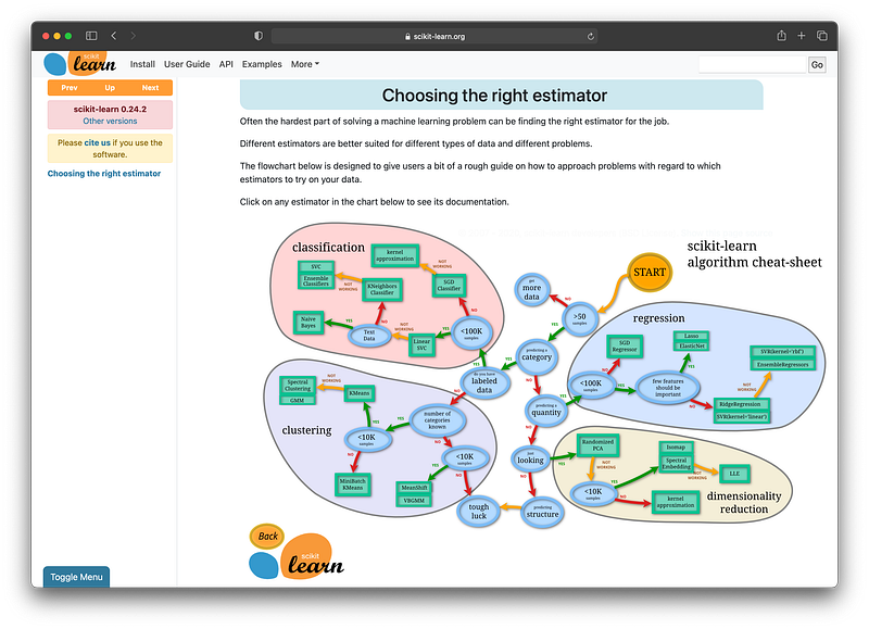
It should be noted that the above image is a preview of the scikit-learn algorithm cheat sheet. To make the most use of this cheat sheet (you can click on the algorithms to see the underlying documentation of the algorithm of interest), proceed to the cheat sheet by going to the link below:

DataCamp

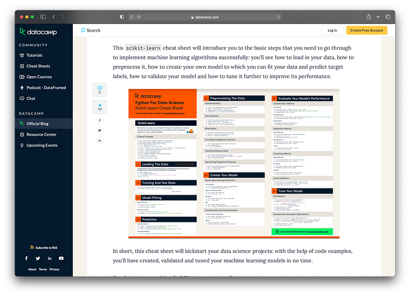
Another useful cheat sheet is the one from DataCamp which provides a printer-friendly one-page form in PDF format as well as a HTML version.

The great thing about this cheat sheet are the code snippets that is provided for various machine learning tasks that can be performed by scikit-learn.

A preview of the cheat sheet is provided below:

The PDF and HTML version of the cheat sheet is available at the link below:

https://www.datacamp.com/community/blog/scikit-learn-cheat-sheet

6.3. Books

Nothing beats some great books at your desk that you can occasionally read or browse through for ideas and inspiration for your projects. Sometimes, I would find a new way of approaching things from examples provided in the book.

Here are some great books covering the usage of scikit-learn that I also personally own and find to be extremely useful.

The Hands-On Machine Learning book by Aurélien Géron is one of the classical books that provides a good coverage of both the concepts and practical sides of implementing machine learning and deep learning models in Python. There is also an appendix section that provide some practical advice on how to set up a machine learning project that may also be helpful for aspiring data scientists.

The author has also shared the Jupyter notebooks of code mentioned in the book on GitHub in this link.

The Python Data Science Handbook by Jake VanderPlas is also another great book that covers some of the important libraries for implementing data science projects. Particularly, the book covers how to use Jupyter notebooks, NumPy, Pandas, Matplotlib and Scikit-learn.

A free online version of the book is also available here. Another gem are the Jupyter notebooks mentioned in the book which is provided on GitHub here.

Conclusion

Congratulations on reaching the end of this article, which also marks the beginning of the myriad of possibilities for exploring data science with scikit-learn.

I hope that you’ve found this article helpful in your data science journey and please feel free to drop a comment to let me know if I’ve left out any approaches or resources in scikit-learn that have been instrumental in your own data science journey.

Disclosure

• As an Amazon Associate, I may earn from qualifying purchases, which goes into helping the creation of future contents.

Read These Next

• How to Master Python for Data Science Here’s the Essential Python you Need for Data Science
• How to Master Pandas for Data Science Here’s the Essential Pandas you Need for Data Science
• How to Build an AutoML App in Python Step-by-Step Tutorial using the Streamlit Library
• Strategies for Learning Data Science Practical Advice for Breaking into Data Science
• How to Build a Simple Portfolio Website for FREE Step-by-step tutorial from scratch in less than 10 minutes

✉️ Subscribe to my Mailing List for my best updates (and occasionally freebies) in Data Science!

About Me

I work full-time as an Associate Professor of Bioinformatics and Head of Data Mining and Biomedical Informatics at a Research University in Thailand. In my after work hours, I’m a YouTuber (AKA the Data Professor) making online videos about data science. In all tutorial videos that I make, I also share Jupyter notebooks on GitHub (Data Professor GitHub page).

Connect with Me on Social Network

✅ YouTube: http://youtube.com/dataprofessor/ ✅ Website: http://dataprofessor.org/ (Under construction) ✅ LinkedIn: https://www.linkedin.com/company/dataprofessor/ ✅ Twitter: https://twitter.com/thedataprof/ ✅ FaceBook: http://facebook.com/dataprofessor/ ✅ GitHub: https://github.com/dataprofessor/ ✅ Instagram: https://www.instagram.com/data.professor/