How To Manipulate Data With DataFrames.jl

A quick tutorial on how to work with data in Julia with DataFrames.jl

Introduction

While Julia might be a programming language that has exploded in popularity recently, a great test of a data science ecosystem in a particular language is usually seeing how well data can be handled and manipulated. One contribution that certainly makes approaching such a problem objectively easier is DataFrames.jl.

notebook

DataFrames.jl is JuliaData’s take on a functional, easy-to-use, and SQL-like data frame management inside of the Julia programming language. Although DataFrames.jl is a rather young package, it frequently gets the job done far better than many of its competitors. That being said, it certainly might take some getting used to. If you also enjoy Python, I wrote another article that will get you familiar with a package called Pandas that is as essential to Python DS as DataFrames.jl is to Julia DS:

The DataFrame Type

As with Pandas, the most important thing that you might want to familiarize yourself with from DataFrames.jl is the DataFrame type. The DataFrame type can be used with several different methods from Julia’s base, as well as some IJulia methods and unique methods for DataFrames. That being said, let’s get started using it! The first step is of course to import DataFrames.jl:

using DataFrames

Whenever the DataFrames package is loaded, the DataFrame type will be exported. We can view the documentation for this type by using the ?() method:

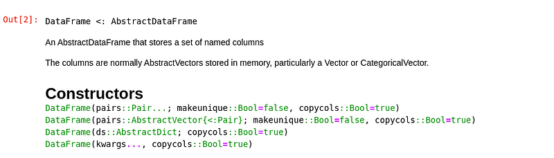
Here we see another cool thing about Julia in the works, as well, abstraction. If you would like to read more about Julia’s handling of abstraction and the inheritance of methods, I wrote an entire article you can check out here!:

Back on topic, we can now construct a DataFrame with any of the constructors listed above, for example with a tuple of pairs:

tuples = (:H => [5, 10], :J => [10, 15])
df = DataFrame(tuples)

Alternatively, we could do the same with a dictionary:

df = DataFrame(dict)

You can also use the DataFrames module with a sink argument to read DataFrames in from various different data sources, such as comma separated values (CSV.)

using DataFrames; df = CSV.read("car data.csv", DataFrame)

If you’d like to read more about sink arguments, I also have an article written all about those, as well that might interest you! :

Our new dataframe can use many base methods, most useful of which is probably push!(), which can be used for concatenation. This will concatenate the observations provided separately, and can be used for logging initial observations.

df = DataFrame(:X => [5,10,15,20], :Y => [5,10,15,20])

push!(df, [10, 15])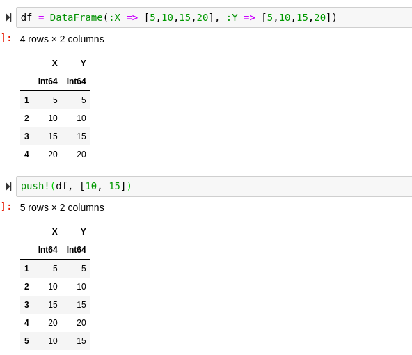

We can access columns on our new DataFrame by either using the child of the struct, or calling the data’s corresponding key.

# Child of struct:
df.X

# Key:
df[!, :X]

We can also get all of the available keys by using the names() function for strings, and propertynames() if we want the same data format used to hold the keys:

names(df)
propertynames(df) 

Finally, we can create a new column by simply assigning a new column equal to something:

df[!, :Z] = [1, 2, 3, 4, 5]

Standard Usage

Now that we are familiar with the DataFrame type, we might want to look at all of the cool functions that we now have access to use on our type. In order to show a DataFrame, you can use the show() method. You might notice that this might not print a full DataFrame, for that you can use the allcols key-word argument:

show(df)
show(df, allcols = true)

We can also do the equivalent of df.head() and df.tail() from Pandas. The equivalent methods are first() and last() respectively:

first(df, 2)

last(df, 3)

Another thing to note is that DataFrames.jl has array-like indexing. This means that often DataFrame calls can be treated like matrix calls, for example:

df[2:4, :]

We can also use Not() to negate any data that we don’t want to include:

df[Not(2:4), :]

We can think of the [:]’s above as *’s in computer language. The colon signifies a selection of all. The first dimension is rows and the second dimension is columns. Taking a look at our data, calling our df at [2, 2] should yield 10.

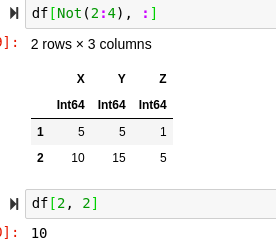
df[2, 2]

10

Joins and Shaping

Often when working with Data Science and data manipulating operations, simple matrix math might not be the only tool required to achieve a good result. DataFrames.jl has SQL-style inner and outer joins, and can typically accomplish most operations with great results.

df2 = DataFrame(:A => [5, 10, 15, 20, 25], :Y => [5, 10, 15, 20, 15])
innerjoin(df, df2, on = :Y)

Of course, you can always identify the usable methods on the DataFrame documentation and utilize the ?() method. There are also left, right, semi, and anti-joins in DataFrames.jl. These are a great way to creatively and functionally manipulate our data.

DataFrames also have another attribute called shape. Shape is a set of two numbers that represent the dimensions of the DataFrame. We can see a DataFrame’s by showing it just as we usually would, with the show() method:

show(df)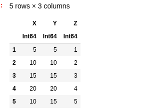

The shape of this DataFrame is 5 x 3, indicated by the 5 rows and three columns. We can manipulate DataFrames using cross-tabulations, pivot-tables, and stacking in order to dramatically alter their shape effectively.

stack(df)

unstack(df)

Data Cleaning

Some of the most important skills for working with large datasets as a Data Scientist is data cleaning skills. These are a little less polished in Julia compared to many of its counterparts such as Pandas, but Julia has some great base methods and data types that will help us get through it!

Firstly, we can use the sort() and sort!() methods respectively in order to sort our data for algorithm optimization and analysis. This is especially valuable in linear analysis situations. In Julia, “ missing” is the data-type that represents a value of data that hasn’t been found and “ nothing” is the data-type used to represent constructors that have not been found.

The best way to remove missing values in Base Julia is to use the skipmissing() method from Julia’s base. This will return a data-efficient iterator that will remove missing data effectively. In Julia, we would then wrap this in the collect method to collect the return of the iterator:

collect(skipmissing(x))

Using DataFrames, we can drop missings with the dropmissing() method. This is a simple and effective way to eliminate missing values from a DataFrame very quickly and effectively over many different features and observations. It also has dispatch for DataFrame columns, so we could work with columns individually if desired:

df = DataFrame(:A => [5, missing, 6], :B => [5, 10, 2])
dropmissing(df)
dropmissing(df, :A)

Conclusion

To conclude, while Julia might not have the most mature package ecosystem underneath its belt, DataFrames.jl is certainly a fantastic package that is well worth using in the Julia language. DataFrames.jl is a valuable asset in a multitude of ways such as allowing SQL-like joins, data visualization, sorting, and most certainly allowing the effective removal of missing data from entire DataFrames. Beyond this, learning how to work with categorical and continuous arrays using methods like push!(), append!(), sort!(), and filter!() and just about anything should easily be handled with DataFrames.jl and Julia together!