
How to Get the Most of the ML Ensembles
Lessons from Kaggle: Compare ensembles algorithms in terms of model accuracy, robustness, and generalization. Implementation included!
Introduction
We previously discussed some of the common ways to leverage the prediction power of Machine Learning (ML) models. These methods are mainly utilized to improve model generalizability by splitting the data into particular schemes.
However, there are more advanced methods to enhance the models’ performance such as ensemble algorithms. In this post, we will discuss and compare the performance of multiple ensemble algorithms. So, let’s get started!
The ensemble method aims to combine the predictions of multiple base-estimator , instead of a single estimator, that leverage the generalization and robustness of the model.
Update 02/13/2021: include the StackingClassifier() class link within the sklearn.ensemble module.
Pre-requisites
- I will use the toy dataset from the UCIML public repository which is hosted on Kaggle; It has nine columns, including the target variable. The notebook is hosted on GitHub if you would like to follow along.
- I utilized the Kaggle API to fetch the dataset while working on the notebook. If you don’t have an account on Kaggle, just download the dataset on your local machine and skip this part in the notebook. You can follow this post on StackOverflow for step-by-step instructions.
I included the script to fetch and download the data into google colab, just make sure you generate your own token before running it.
3. I did some basic preprocessing to the dataset before building the model — such as imputing missing data, to avoid errors.
4. I created two separate notebooks, one for comparing the first three ensembles. The second one comprises the implementation of the stacked ensemble from scratch and using the MLens library.
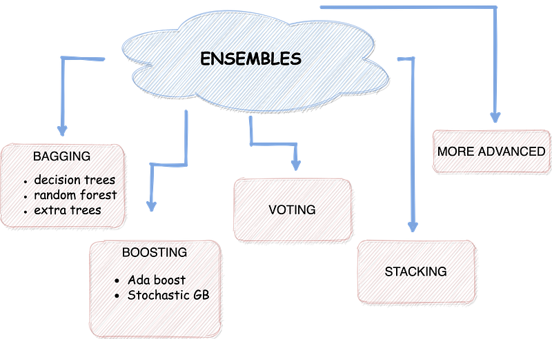
Methods of ensembles
Ensembles are procedures that build various models and then blend them to produce improved predictions. Ensembles enable achieving more precise predictions compared to a single model. Utilizing Ensembles typically gave the edge for the winning teams in ML competitions. You can find the CrowdFlower winners’ interview — Team Quartet, who used Ensemble to win the competition.
1. Bagging — Bootstrap Aggregating:
Bootstrap aggregating tends to build multiple models (using the same type of algorithms) from different subsamples with replacement from the training dataset.
Bagging is to ensemble several good models to reduce the model variance.
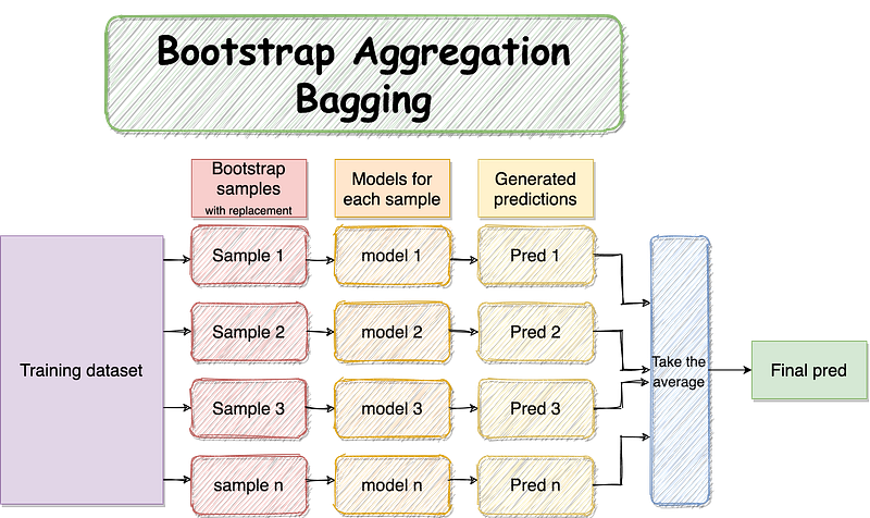
Bagging has three types of ensembles as follows:
1.2 Bagging decision trees
Bagging performs best with algorithms that produce high variance predictions. In the following example, we will develop the BaggingClassifier() combined with a DecisionTreeClassifier() within the sklearn library.
Please note that the results may differ due to stochastic learning nature!
Bagging produces models and splits the samples in parallel.
from sklearn.ensemble import BaggingClassifiertree = DecisionTreeClassifier()
bagging_clf = BaggingClassifier(base_estimator=tree, n_estimators=1500, random_state=42)
bagging_clf.fit(X_train, y_train)
evaluate(bagging_clf, X_train, X_test, y_train, y_test)TRAINIG RESULTS:
===============================
CONFUSION MATRIX:
[[350 0]
[ 0 187]]
ACCURACY SCORE:
1.0000
CLASSIFICATION REPORT:
0 1 accuracy macro avg weighted avg
precision 1.0 1.0 1.0 1.0 1.0
recall 1.0 1.0 1.0 1.0 1.0
f1-score 1.0 1.0 1.0 1.0 1.0
support 350.0 187.0 1.0 537.0 537.0
TESTING RESULTS:
===============================
CONFUSION MATRIX:
[[126 24]
[ 38 43]]
ACCURACY SCORE:
0.7316
CLASSIFICATION REPORT:
0 1 accuracy macro avg weighted avg
precision 0.768293 0.641791 0.731602 0.705042 0.723935
recall 0.840000 0.530864 0.731602 0.685432 0.731602
f1-score 0.802548 0.581081 0.731602 0.691814 0.724891
support 150.000000 81.000000 0.731602 231.000000 231.0000001.2 Random Forest (RF)
Random Forest (RF) is a meta estimator that fits different decision tree classifiers on multiple sub-samples and estimates the average accuracy.
The sub-sample size is constant, but the samples are drawn with replacement if bootstrap=True (default).
Now, let’s take a shot and try the Random forest (RF) model. RF works like the bagged decision tree class; however, it reduces the correlation between individual classifiers. RF only considers the random subset of features per split instead of following the greedy approach to picking the best split point.
from sklearn.ensemble import RandomForestClassifier

rf_clf = RandomForestClassifier(random_state=42, n_estimators=1000)
rf_clf.fit(X_train, y_train)
evaluate(rf_clf, X_train, X_test, y_train, y_test)
TRAINIG RESULTS:
===============================
CONFUSION MATRIX:
[[350 0]
[ 0 187]]
ACCURACY SCORE:
1.0000
CLASSIFICATION REPORT:
0 1 accuracy macro avg weighted avg
precision 1.0 1.0 1.0 1.0 1.0
recall 1.0 1.0 1.0 1.0 1.0
f1-score 1.0 1.0 1.0 1.0 1.0
support 350.0 187.0 1.0 537.0 537.0
TESTING RESULTS:
===============================
CONFUSION MATRIX:
[[127 23]
[ 38 43]]
ACCURACY SCORE:
0.7359
CLASSIFICATION REPORT:
0 1 accuracy macro avg weighted avg
precision 0.769697 0.651515 0.735931 0.710606 0.728257
recall 0.846667 0.530864 0.735931 0.688765 0.735931
f1-score 0.806349 0.585034 0.735931 0.695692 0.728745
support 150.000000 81.000000 0.735931 231.000000 231.0000001.3 Extra trees — ET
Extra Trees (ET) is a modification of bagging. The ExtraTreesClassifier() is a class from the sklearn library that creates a meta estimator to fit several randomized decision trees (a.k.a. ET) of various sub-samples. Then, ET computes the average prediction among the sub-samples. This allows improving the accuracy of the model and control for over-fitting.
from sklearn.ensemble import ExtraTreesClassifier

ex_tree_clf = ExtraTreesClassifier(n_estimators=1000, max_features=7, random_state=42)
ex_tree_clf.fit(X_train, y_train)
evaluate(ex_tree_clf, X_train, X_test, y_train, y_test)
TRAINIG RESULTS:
===============================
CONFUSION MATRIX:
[[350 0]
[ 0 187]]
ACCURACY SCORE:
1.0000
CLASSIFICATION REPORT:
0 1 accuracy macro avg weighted avg
precision 1.0 1.0 1.0 1.0 1.0
recall 1.0 1.0 1.0 1.0 1.0
f1-score 1.0 1.0 1.0 1.0 1.0
support 350.0 187.0 1.0 537.0 537.0
TESTING RESULTS:
===============================
CONFUSION MATRIX:
[[124 26]
[ 32 49]]
ACCURACY SCORE:
0.7489
CLASSIFICATION REPORT:
0 1 accuracy macro avg weighted avg
precision 0.794872 0.653333 0.748918 0.724103 0.745241
recall 0.826667 0.604938 0.748918 0.715802 0.748918
f1-score 0.810458 0.628205 0.748918 0.719331 0.746551
support 150.000000 81.000000 0.748918 231.000000 231.0000002. Boosting
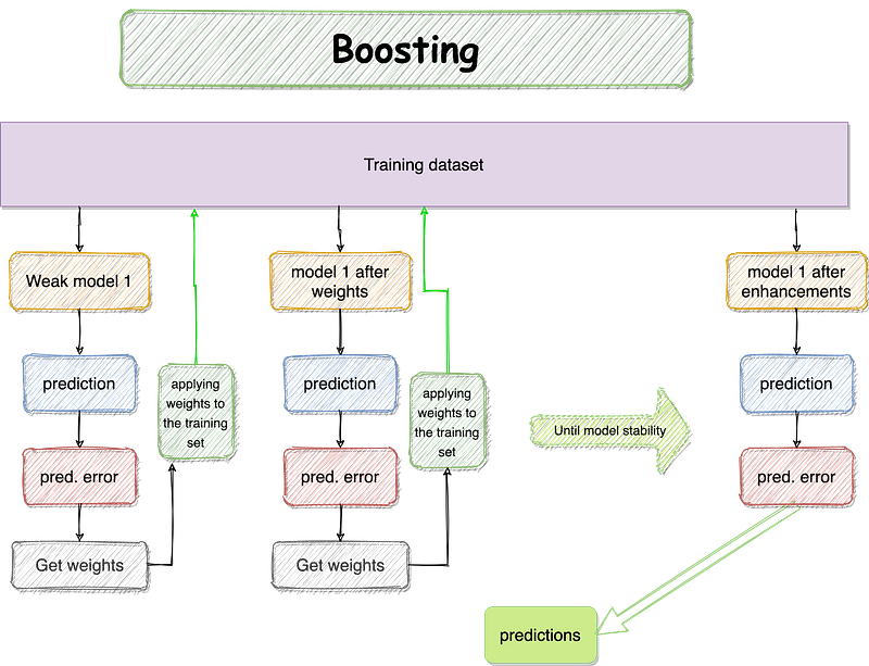
Boosting is another technique to build multiple models (also from the same type); however, each model learns to fix the previous model’s prediction errors across the models’ sequence. Boosting is primarily used to balance the bias and variance in the supervised machine learning models. Boosting is an algorithm that converts weak learners into strong ones.
Boosting manages to build a base estimator sequentially from weak ones, then reduce the combined estimators’ bias.
2.1 AdaBoost (AD)
AdaBoost (AD) weighs the dataset instances by classifying features. This enables the algorithm to account for these features in constructing the subsequent model.
from sklearn.ensemble import AdaBoostClassifier

ada_boost_clf = AdaBoostClassifier(n_estimators=30)
ada_boost_clf.fit(X_train, y_train)
evaluate(ada_boost_clf, X_train, X_test, y_train, y_test)
TRAINIG RESULTS:
===============================
CONFUSION MATRIX:
[[314 36]
[ 49 138]]
ACCURACY SCORE:
0.8417
CLASSIFICATION REPORT:
0 1 accuracy macro avg weighted avg
precision 0.865014 0.793103 0.841713 0.829059 0.839972
recall 0.897143 0.737968 0.841713 0.817555 0.841713
f1-score 0.880785 0.764543 0.841713 0.822664 0.840306
support 350.000000 187.000000 0.841713 537.000000 537.000000
TESTING RESULTS:
===============================
CONFUSION MATRIX:
[[129 21]
[ 36 45]]
ACCURACY SCORE:
0.7532
CLASSIFICATION REPORT:
0 1 accuracy macro avg weighted avg
precision 0.781818 0.681818 0.753247 0.731818 0.746753
recall 0.860000 0.555556 0.753247 0.707778 0.753247
f1-score 0.819048 0.612245 0.753247 0.715646 0.746532
support 150.000000 81.000000 0.753247 231.000000 231.0000002.2 Stochastic Gradient Boosting ( SGB )
Stochastic Gradient Boosting (SGB) is one of the advanced ensemble algorithms. At each iteration, SGB randomly draws a sub-sample from the training set (without replacement). The sub-sample is then utilized to fit the base model(learner) until the error becomes stable.
from sklearn.ensemble import GradientBoostingClassifier

grad_boost_clf = GradientBoostingClassifier(n_estimators=100, random_state=42)
grad_boost_clf.fit(X_train, y_train)
evaluate(grad_boost_clf, X_train, X_test, y_train, y_test)
TRAINIG RESULTS:
===============================
CONFUSION MATRIX:
[[339 11]
[ 26 161]]
ACCURACY SCORE:
0.9311
CLASSIFICATION REPORT:
0 1 accuracy macro avg weighted avg
precision 0.928767 0.936047 0.931099 0.932407 0.931302
recall 0.968571 0.860963 0.931099 0.914767 0.931099
f1-score 0.948252 0.896936 0.931099 0.922594 0.930382
support 350.000000 187.000000 0.931099 537.000000 537.000000
TESTING RESULTS:
===============================
CONFUSION MATRIX:
[[126 24]
[ 37 44]]
ACCURACY SCORE:
0.7359
CLASSIFICATION REPORT:
0 1 accuracy macro avg weighted avg
precision 0.773006 0.647059 0.735931 0.710032 0.728843
recall 0.840000 0.543210 0.735931 0.691605 0.735931
f1-score 0.805112 0.590604 0.735931 0.697858 0.729895
support 150.000000 81.000000 0.735931 231.000000 231.0000003. Voting
Voting is a set of equally well-performing models to balance out their weaknesses. Voting uses three approaches for the voting procedure, hard, soft, and weighted.
- Hard voting — the majority of class labels predicted.
- Soft voting — the argmax of the sum of predicted probabilities.
- Weighted voting — the argmax of the weighted sum of predicted probabilities.
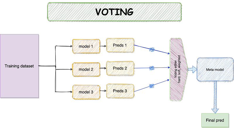
Voting is simple and easy to implement. First, it creates two standalone models (may be more depending on the use case) from the dataset. A voting classifier is then used to wrap the models and average the submodels’ predictions when introducing the new data.
from sklearn.ensemble import VotingClassifier
from sklearn.linear_model import LogisticRegression
from sklearn.svm import SVC

estimators = []
log_reg = LogisticRegression(solver='liblinear')
estimators.append(('Logistic', log_reg))

tree = DecisionTreeClassifier()
estimators.append(('Tree', tree))

svm_clf = SVC(gamma='scale')
estimators.append(('SVM', svm_clf))

voting = VotingClassifier(estimators=estimators)
voting.fit(X_train, y_train)

evaluate(voting, X_train, X_test, y_train, y_test)
TRAINIG RESULTS:
===============================
CONFUSION MATRIX:
[[328 22]
[ 75 112]]
ACCURACY SCORE:
0.8194
CLASSIFICATION REPORT:
0 1 accuracy macro avg weighted avg
precision 0.813896 0.835821 0.819367 0.824858 0.821531
recall 0.937143 0.598930 0.819367 0.768037 0.819367
f1-score 0.871182 0.697819 0.819367 0.784501 0.810812
support 350.000000 187.000000 0.819367 537.000000 537.000000
TESTING RESULTS:
===============================
CONFUSION MATRIX:
[[135 15]
[ 40 41]]
ACCURACY SCORE:
0.7619
CLASSIFICATION REPORT:
0 1 accuracy macro avg weighted avg
precision 0.771429 0.732143 0.761905 0.751786 0.757653
recall 0.900000 0.506173 0.761905 0.703086 0.761905
f1-score 0.830769 0.598540 0.761905 0.714655 0.749338
support 150.000000 81.000000 0.761905 231.000000 231.0000004. Stacking
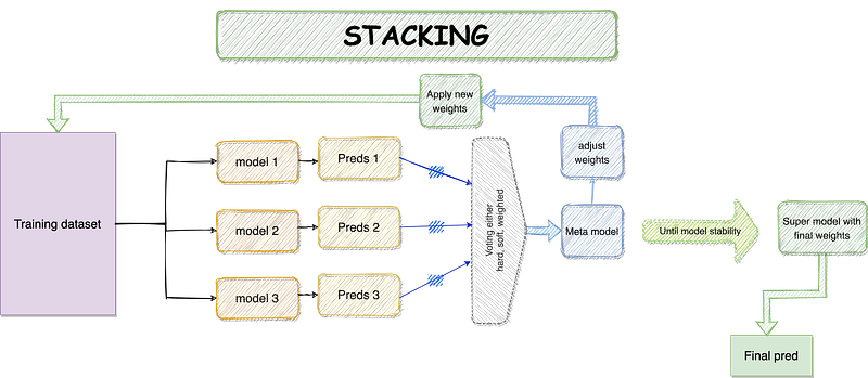
Stacking has the same working principle as the voting ensemble. However, stacking can control the ability to adjust the submodels’ predictions sequentially- as inputs to the meta-model, to boost the performance. In other words, stacking generates predictions from each model’s algorithm; subsequently, the meta-model uses these predictions as inputs (weights) to create the final outputs.
The superiority of stacking is that it can combine different powerful learners and make precise and robust predictions than any standalone model.
The sklearn library has the StackingClassifier() under the ensemble module, you can find the link here. However, I will implement the stacking ensemble using the ML-Ensemble library.
To make a fair comparison between stacking and the previous ensembles, I recalculated the previous accuracies using a fold of 10.
from mlens.ensemble import SuperLearner# create a list of base-models
def get_models():
models = list()
models.append(LogisticRegression(solver='liblinear'))
models.append(DecisionTreeClassifier())
models.append(SVC(gamma='scale', probability=True))
models.append(GaussianNB())
models.append(KNeighborsClassifier())
models.append(AdaBoostClassifier())
models.append(BaggingClassifier(n_estimators=10))
models.append(RandomForestClassifier(n_estimators=10))
models.append(ExtraTreesClassifier(n_estimators=10))
return modelsdef get_super_learner(X):
ensemble = SuperLearner(scorer=accuracy_score,
folds = 10,
random_state=41)
model = get_models()
ensemble.add(model)
# add some layers to the ensemble structure
ensemble.add([LogisticRegression(), RandomForestClassifier()])
ensemble.add([LogisticRegression(), SVC()])
# add meta model
ensemble.add_meta(SVC())
return ensemble# create the super learner
ensemble = get_super_learner(X_train)
# fit the super learner
ensemble.fit(X_train, y_train)
# summarize base learners
print(ensemble.data)
# make predictions on hold out set
yhat = ensemble.predict(X_test)
print('Super Learner: %.3f' % (accuracy_score(y_test, yhat) * 100))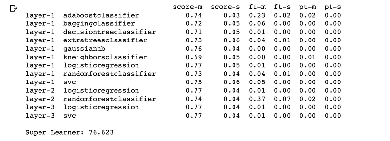
ACCURACY SCORE ON TRAIN: 83.24022346368714
ACCURACY SCORE ON TEST: 76.62337662337663
Compare the performance
import plotly.graph_objects as gofig = go.Figure()
fig.add_trace(go.Bar(
x = test['Algo'],
y = test['Train'],
text = test['Train'],
textposition='auto',
name = 'Accuracy on Train set',
marker_color = 'indianred'))fig.add_trace(go.Bar(
x = test['Algo'],
y = test['Test'],
text = test['Test'],
textposition='auto',
name = 'Accuracy on Test set',
marker_color = 'lightsalmon'))fig.update_traces(texttemplate='%{text:.2f}')
fig.update_layout(title_text='Comprehensive comparasion between ensembles on Train and Test set')
fig.show()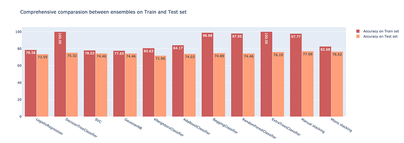
As shown, the stacked ensemble performed great on the test set, with the highest classification accuracy is 76.623%. Great!
4. Conclusions and Takeaways
We have explored several types of ensembles and learned to implement them the right way to extend the model’s predictive power. We’ve also concluded some essential points to consider:
- Stacking showed improvement in the accuracy, robustness and got a better generalization.
- We may use voting in such cases when we want to set equally well-performing models to balance their weaknesses.
- Boosting is a great ensemble; It merely combines multiple weak learners to get a powerful one.
- You may consider Bagging when you want to produce a model with less variance by combining different good models — decrease overfitting.
- Choosing the right ensemble depends on the business problem and what outcome you desire.
Finally, I wish this gave a comprehensive guide on implementing ensembles and get the most out of them. If you encountered any issues, please list them in the comment section; I would be happy to help. The best way to encourage me is by following me here on Medium, LinkedIn, or Github. Happy learning!