How to Find Optimal Neural Network Architecture with TensorFlow — The Easy Way

Your go-to guide for optimizing feed-forward neural network models on any dataset

Deep learning boils down to experimentation. Training hundreds of models by hand is tedious and time-consuming. I’d rather do something else with my time, and I imagine the same holds for you.

Picture this — you want to find the optimal architecture for your deep neural network. Where do you start? How many layers? How many nodes per layer? What about the activation functions? There are just too many moving parts.

You can automate this process to a degree, and this article will show you how. After reading, you’ll have one function for generating neural network architectures given specific parameters and the other one for finding the optimal architecture.

Don’t feel like reading? Watch my video instead:

You can download the source code on GitHub.

Dataset used and data preprocessing

I don’t plan to spend much time here. We’ll use the same dataset as in the previous article — the wine quality dataset from Kaggle:

You can use the following code to import it to Python and print a random couple of rows:

We’re ignoring the warnings and changing the default TensorFlow log level just so we don’t get overwhelmed with the output.

Here’s how the dataset looks like:

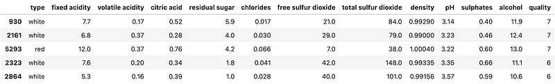
The dataset is mostly clean, but isn’t designed for binary classification by default (good/bad wine). Instead, the wines are rated on a scale. We’ll address that now, with numerous other things:

• Delete missing values — There’s only a handful of them, so we won’t waste time on imputation.
• Handle categorical features — The only one is type, indicating whether the wine is white or red.
• Convert to a binary classification task — We’ll declare any wine with a grade of 6 and above as good, and anything below as bad.
• Train/test split — A classic 80:20 split.
• Scale the data — The scale between predictors differs significantly, so we’ll use the StandardScaler to bring the values closer.

Here’s the entire data preprocessing code snippet:

Once again, please refer to the previous article if you want more detailed insights into the logic behind data preprocessing.

With that out of the way, let’s see how to approach optimizing neural network architectures.

How to approach optimizing neural network models?

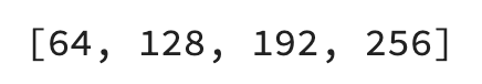
The approach to finding the optimal neural network model will have some tweakable constants. Today’s network will have 3 hidden layers, with a minimum of 64 and a maximum of 256 nodes per layer. We’ll set the step size between nodes to 64, so the possibilities are 64, 128, 192, and 256:

Let’s verify the node number possibilities. You can do so by creating a list of ranges between the minimum and maximum number of nodes, having the step size in mind:

Here’s what you’ll see:

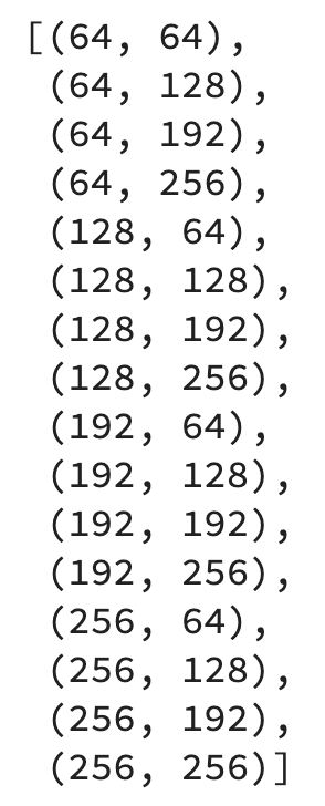
Taking this logic to two hidden layers, you end up with the following possibilities:

Or visually:

To get every possible permutation of the options among two layers, you can use the product() function from itertools:

Here’s the output:

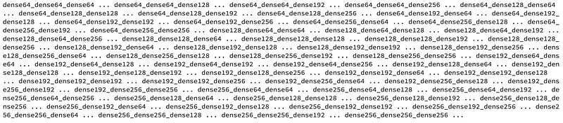
The goal is to optimize a 3-layer-deep neural network, so we’ll end up with a bit more permutations. You can declare the possibilities by first multiplying the list of node options with num_layers and then calculate the permutations:

It’s a lot of options — 64 in total. During optimization, we’ll iterate over the permutations and then iterate again over the values of the individual permutation to get the node counts for each hidden layer.

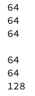
In short, we’ll have two for loops. Here’s the logic for the first two permutations:

The second print statement is here just to make a gap between models, so don’t think too much of it. Here’s the output:

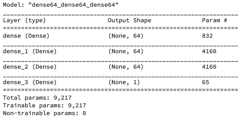
We’ll create a new tf.keras.Sequential model at each iteration and add a tf.keras.layers.InputLayer to it with a shape of a single training row ((12,)). Then, we’ll iterate over the items in a single permutation and add a tf.keras.layers.Dense layer to the model with the number of nodes set to the current value of the single permutation. Finally, we’ll add a tf.keras.layers.Dense output layer.

It’s a good idea to set the name to the model, so it’s easier to compare them later. We’ll hardcode the input shape and the activation functions for no, and set these parts as dynamic in the next section.

Here’s the code:

And now let’s inspect how a single model looks like:

That’s the logic we’ll go with. There’s a way to improve it, though, as it’s not convenient to run dozens of notebook cells every time you want to run the optimization. It’s also not the best idea to hardcode values for activation functions, input shape, and so on.

For that reason, we’ll declare a function for generating Sequential models next.

Model generation function for optimizing neural networks

The function accepts a lot of parameters but doesn’t contain anything we didn’t cover previously. It gives you the option to change the input shape, activation function for the hidden and output layer, and the number of nodes at the output layer.

Here’s the code:

Let’s test it — we’ll stick to a model with three hidden layers, each having a minimum of 64 and a maximum of 256 nodes:

Feel free to inspect the values of the all_models list. It contains 64 Sequential models, each having a unique name and architecture. Training so many models will take time, so let’s make things extra simple by writing yet another helper function.

Model training function for optimizing neural networks

This one accepts the list of models, training and testing data, and optionally a number of epochs and the verbosity level. It’s advised to set verbosity to 0, so you don’t get overwhelmed with the console output. The function returns a Pandas DataFrame containing the performance metrics on the test set, measured in accuracy, precision, recall, and F1.

Here’s the code:

And now, let’s finally start the optimization.

Running the optimization

Keep in mind — the optimization will take some time, as we’re training 64 models for 50 epochs. Here’s how to start the process:

The optimization ran for 34 minutes on my machine (M1 MacBook Pro) and printed the following:

You’re seeing this output because of the print() statement in the optimize() function. It’s there to give you a sense of the progress.

We now have a DataFrame we can sort either by accuracy, precision, recall, or F1. Here’s how to sort it by accuracy in descending order, so the model with the highest value is displayed first:

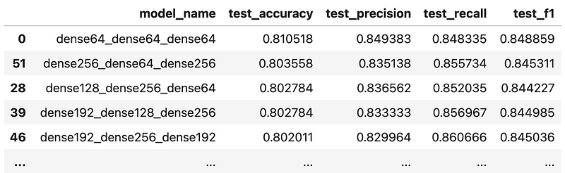
It looks like the simplest model resulted in the best accuracy. You could also test the optimization for models with two and four hidden layers, or even more, but I’ll leave that up to you. It’s just a matter of calling the get_models() function and passing in different parameter values.

And that’s all I wanted to cover today. Let’s wrap things up next.

Parting words

Finding an optimal neural network architecture for your dataset boils down to one thing and one thing only — experimentation. It’s quite tedious to train and evaluate hundreds of models by hand, so the two functions you’ve seen today can save you some time. You still need to wait for the models to train, but the entire process is fast on this dataset.

A good way to proceed from here is to pick an architecture you find best and tune the learning rate.

Things get a lot more complicated and the training times get longer if you’re dealing with image data and convolutional layers. That’s what the next article will cover — we’ll start diving into computer vision and train a simple convolutional neural network. Don’t worry, it won’t be on the MNIST dataset.

How do you approach optimizing feed-forward neural networks? Is it something similar, or are you using a dedicated AutoML library? Please let me know in the comment section below.

Loved the article? Become a Medium member to continue learning without limits. I’ll receive a portion of your membership fee if you use the following link, with no extra cost to you.

Stay connected

• Sign up for my newsletter
• Subscribe on YouTube
• Connect on LinkedIn