How to Evaluate Representations

From unsupervised to supervised metrics

Embeddings, also known as representations, are dense vector representations of entities such as words, documents, products, and more. They are designed to capture semantic meanings and highlight similarities among entities. A good set of representations should not only efficiently encode the essential features of entities but also exhibit properties like compactness, meaningfulness, and robustness across various tasks. In this article, we look into various evaluation metrics to assess the quality of representations. Let’s get started.

An Evaluation Framework

Any evaluation framework consists of three main components:

1. A baseline method: this serves as a benchmark against which new approaches or models are compared. It provides a reference point for evaluating the performance of the proposed methods.
2. A set of evaluation metrics: evaluation metrics are quantitative measures used to evaluate the performance of the models. These metrics can be supervised or unsupervised, and define how the success of the outputs is assessed.
3. An evaluation dataset: the evaluation dataset is a collection of labeled/annotated or unlabelled data used to assess the performance of the models. This dataset should be representative of the real-world scenarios that the models are expected to handle. It needs to cover a diverse range of examples to ensure a comprehensive evaluation.

Based on if evaluation metrics require ground truth labels, we can split them into un-supervised metrics, and supervised metrics. It is often more advantageous to employ un-supervised metrics, as they do not require labels, and the collection of labels is very expensive in practice.

Below, we will look into state-of-the-art metrics. For each metric, pick a baseline method to compare your evaluations against. The baseline can be as simple as `random embedding generator`!

Supervised Evaluation Metrics

Supervised metrics require a labelled evaluation dataset. A common strategy is to choose a predictor such as a classifier or regressor. Then train the predictor on a limited set of labeled data from a specific task. Next, using a supervised metric measure the predictor’s performance on a held-out dataset.

It is worth it to mention two valuable points here:

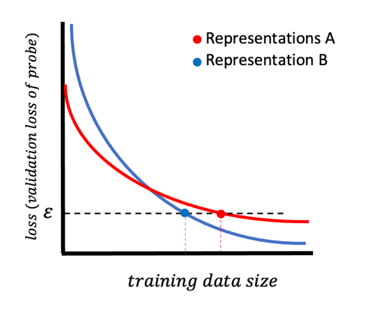
1️⃣ The `validation accuracy`, a commonly used metric, is shown to be sensitive to the size of the dataset used for training the probe[3]!! It is shown that validation accuracy is sensitive to the size of the training dataset; they may choose a different representations for the same task when given dataset of different sizes [3]! Ideally, this assessment must be independent of the dataset size and be only dependent on the data distribution [3].

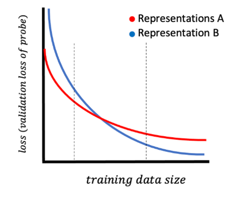
The figure below shows this phenomena: two representations, one in red (representation A), and one in blue (representation B) are shown. The x-axis denotes the size of the training data used to train the predictor (referred to as probe). The y-axis shows the validation loss of the trained probe. Note the probe is trained on representations from each method. As we see, as training data size increases on the x-axis, the validation loss of the probe decreases on the y-axis. However, at some point, the two loss curves cross each other!! Therefore in small data sizes, representation A has lesser loss, while in larger data sizes the representation B has lesser loss. The paper in[3] names this curve the loss-data curve as it measures the loss of the predictor vs the training data size used to train the probe.

2️⃣ Linear predictors (linear classifiers/regressors) are widely criticized as a method to evaluate representations[4]; it is shown that models that perform strongly on linear classification tasks can perform weakly on more complex tasks [4].

There are many supervised metrics proposed in literature; Mutual Information (MI), F1 score, BLEU, Precision, Recall, Minimum Descriptor Length (MDL) to name a few but the SOTA metrics [3,9] in supervised evaluation realm are Surplus Description Length (SDL) and ϵ−sample complexity.

Surplus Description Length (SDL) and ϵ−sample complexity are inspired by the idea that “the best representation is the one which allows for the most efficient learning of a predictor to solve the task” [3,9]. As [3] mentions “this position is motivated by practical concerns; the more labels that are needed to solve a task in the deployment phase, the more expensive to use and the less widely applicable a representation will be”.

Intuition: To give an intuition, the SDL and ϵ−sample complexity metrics do not measure a quantity on a fixed data size, instead they estimate the loss-data curve and measure quantities with respect to the curve[3]. To that end, for both metrics the user specifies a tolerance ϵ so that a population loss of less than ϵ qualifies as solving the task. An ϵ-loss predictor is then any predictor which achieves loss lesser than ϵ [3]. Then the measures compute the cost of learning a predictor which achieves that loss.

Let’s dive into the details of each metric:

Surplus Description Length (SDL)

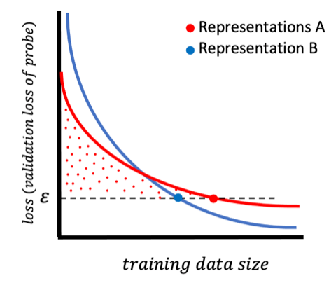
As mentioned in [3], this metric corresponds to computing the area between the loss-data curve and a baseline set by y = ϵ. In other words, it measures the cost of re-creating an ϵ-loss predictor using the representation [3]. Mathematically, it is defined as following

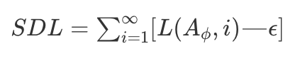
Here, A is an algorithm, it can be any predicting algorithm such as classification or regression, and L(A, i) refers to the loss of this predictor resulting from training algorithm A on the first i data points [3]. Naively computing this metric require unbounded data so in practice it is always estimated [3]. For an implementation of this metric refer to the Github repository at [8].

ϵ−sample complexity

As mentioned in [3], this metric measures the complexity of learning an ϵ-loss predictor by the number of samples it takes to find it. It is defined as:

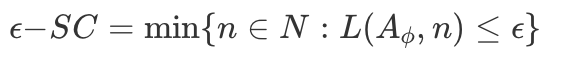
This measures allows the comparison of two representation by first picking a target function to learn (e.g., an epsilon loss 2 layer MLP classifier) then measuring which representations enables learning that function with less data [3].

Unsupervised Evaluation Metrics:

These metrics are every scientist’s favorite as they do not require labelled data. Some examples of common unsupervised metrics are the followings:

1) Cluster Learnability (CL):

This metric[1] assesses the learnability of representations. A higher Cluster Learnability (CL) score indicates that the learned representation is better at separating different clusters in the input data space. CL is measured as the learning speed of a K-Nearest Neighbor (KNN) classifier trained to predict labels obtained by clustering the representations with K-means.

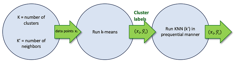
It consists of three main steps and works as following:

1. Pick hyper-parameters k=number of clusters and k′ = number of neighbors. Let x_i​ denote the representations of i−th data point.
2. Run k-means on the dataset to obtain k clusters; assign cluster id to each datapoint x_i​ as its label. Denote it as y^_i$​.
3. Run KNN in a prequential manner on each datapoint to obtain a predicted label by majority rule. If a datapoint is {x_i​, y_​i}​ take all data points numbered lesser than i i.e {x_j​ | j

Then the Cluster Learnability (CL) metric would be

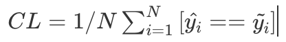
The intuition for this metric is as following: The “prequential” approach is a way of evaluating the performance of a machine learning model, such as KNN, in an online learning setting. In this context, “prequential” combines the words “predictive” and “sequential.” In the prequential manner of KNN computation, the model is evaluated and updated sequentially, one instance at a time, using a stream of data. Since the data is unlabeled, this method uses clustering in step 2 to synthetically generate labels (i.e. cluster ids) and use them to compute the speed of cluster learnability in an online (prequential) manner.

The following code computes this metric :

2) Silhouette Coefficient

Similar to CL metric, silhouette coefficient metric measures clusterability of entities that inherently belong to one cluster. This metric measures the quality of clusters through their cohesion and separation. In other words, it measures how well each sample in a cluster is separated from samples in other clusters, and provides an indication of how compact and well-separated the clusters are. The Silhouette Coefficient ranges from -1 to 1:

• A value close to 1 indicates that samples are well-clustered and far from samples in neighboring clusters.
• A value close to 0 suggests overlapping clusters or samples that are on or very close to the decision boundary between clusters.
• A value close to -1 indicates that samples are likely assigned to the wrong clusters.

The following code computes this metric :

3) Cluster Purity

This metric evaluates the quality of clusters obtained from representations. It measures the extent to which clusters contain data points from a single class. The steps to compute cluster purity are:

1. For each cluster, identify the majority class in that cluster. Count the number of data points of the majority class in each cluster.
2. Sum these counts for all clusters. Divide the sum by the total number of data points.

The value ranges from 0 to 1. Higher values indicate better clusters, with 1 being perfect clustering where each cluster contains solely points from one class.

The following code computes this metric :

Summary

It’s imperative to assess quality of representations before feeding them into any machine learning model. To evaluate their quality we must have a framework consisting of three components: a baseline method, evaluation metrics, and an evaluation datasets. Metric divide into supervised and unsupervised, based on if they need a labelled dataset or not. Often unsupervised metrics are advantageous as they don’t require labelled dataset and collecting/curating label is difficult and time-consuming. The unsupervised metrics include cluster purity, cluster-ability and cluster-learnability. On the other hand, the state of the art supervised metrics are surplus descriptor length (SDL) and ϵ-sample complexity. Regardless of the choice of the metric, it’s important to stay consistent and use one single metric to compare two set of representations against each other.

If you have any questions or suggestions, feel free to reach out to me: Email: [email protected] LinkedIn: https://www.linkedin.com/in/minaghashami/

References

1. Expressiveness and Learnability: A Unifying View for Evaluating Self-Supervised Learning
2. Self-Supervised Representation Learning: Introduction, Advances and Challenges
3. Evaluating representations by the complexity of learning low-loss predictors
4. Probing the State of the Art: A Critical Look at Visual Representation Evaluation
5. Representation learning with contrastive predictive coding
6. Learning representations by maximizing mutual information across views
7. On mutual information maximization for representation learning
8. https://github.com/willwhitney/reprieve