
How to Effectively Forecast Time Series with Amazon's New Time Series Forecasting Model
Learn about the new Amazon time series model, which you can use to forecast energy usage, traffic congestion, and weather.
I will discuss Amazon's new Chronos time series forecasting model [1]. The model can be used for a variety of time series forecasting tasks, such as predicting energy usage, traffic/congestion forecasting, or weather prediction. This makes it both flexible and powerful. I will discuss the model's performance, strengths and weaknesses, and how you can implement and run it locally.

Motivation
The motivation for this article is to follow up on the latest models within machine learning. I learned about this model from looking at PapersWithCode, one of the sources I consistently check to keep up with the latest trends in machine learning. Whenever I find something interesting, I like implementing it and getting a feel for the model and its performance. This article will discuss how you can use this model yourself, which tasks you can apply the model to, and my thoughts on the performance of the model.
After running the model, you will be able to make forecasts for the model, like in the image you see below:
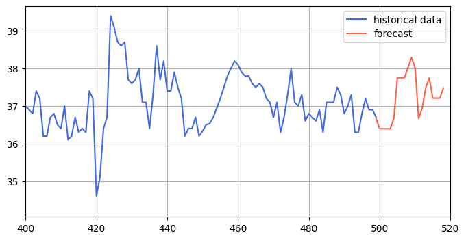
Table of contents
· Motivation · Implementing the model · Tasks you can use the model for · Dataset · Accuracy measurements · Testing the model · My thoughts on the model · Future work · Conclusion · References
Implementing the model
The README from the Chronos time series' official GitHub page thoroughly explains how to implement the model. However, I will also explain how I use the model using my own functions based on the code in GitHub.
First, you must download the Chronos package, which you can do with the following command:
pip install git+https://github.com/amazon-science/chronos-forecasting.git
Then, you must download PyTorch from the official website. If you want to use the GPU with CUDA, which I do in the code later, you must download it with the GPU.
If not downloaded already with PyTorch, you also need:
pip install pandas
pip install numpy
pip install tqdm
Then you can import all the required packages:
import matplotlib.pyplot as plt
import numpy as np
import pandas as pd
import torch
from chronos import ChronosPipeline
from tqdm.auto import tqdm
And then download the model:
pipeline = ChronosPipeline.from_pretrained(
  "amazon/chronos-t5-base",
  device_map="cuda",
  torch_dtype=torch.bfloat16,
)
On Windows, the code above will download the model to the folder path: C:\Users\<user>\.cache\huggingface\hub. If you want to move the model somewhere else and use it, you can change the code above to:
pipeline = ChronosPipeline.from_pretrained(
  "<path where you store model>",
  device_map="cuda",
  torch_dtype=torch.bfloat16,
)
Where <path where you store model> is the path you moved your model to. It also works to directly link to another device here if you are, for example, working on an external SSD.
I then use the following three functions to use the model:
def load_model():
 pipeline = ChronosPipeline.from_pretrained(
 "amazon/chronos-t5-base",
 device_map="cuda",
 torch_dtype=torch.bfloat16,
 )
 return pipeline

def predict(pipeline, timeseries, prediction_length=12):
 """given a timeseries, predict with chronos model"""
 forecast = pipeline.predict(timeseries, prediction_length, num_samples=1)[0][0]  # shape [num_series, num_samples, prediction_length]
 return forecast

def visualize(timeseries, forecast, ground_truth=None, xlim=None, ylim=None):
 # visualize the forecast
 assert isinstance(timeseries, torch.Tensor) and isinstance(forecast, torch.Tensor), "timeseries and forecast should be numpy arrays"

 plt.figure(figsize=(8, 4))
 plt.plot(range(len(timeseries)), timeseries, color="royalblue", label="historical data")
 plt.plot(range(len(timeseries)-1, len(timeseries) - 1 + len(forecast)), forecast, color="tomato", label="forecast")
 if ground_truth is not None:
  plt.plot(range(len(timeseries)-1, len(timeseries) - 1 + len(ground_truth)), ground_truth, color="green", label="ground truth")
 if xlim is not None:
  plt.xlim(xlim)
 if ylim is not None:
  plt.ylim(ylim)
 plt.legend()
 plt.grid()
 plt.show()
You can use this code as an example of linear growth. Given an array [0, 1, 2, …, 97, 98, 99], the model will predict the following ten values, which should naturally be [100, 101, …, 108, 109].
pipeline = load_model()
example_timeseries = torch.tensor(range(100), dtype=torch.float32)
forecast = predict(pipeline, example_timeseries)
Where the forecast is:
[100.1613, 101.2500, 102.3387, 103.0645, 104.1532, 105.2419, 105.9677,
        107.0565, 108.1451, 108.8710, 109.9597, 110.6855]
Which you can visualize with the code:
visualize(example_timeseries, forecast)Which plots the following:
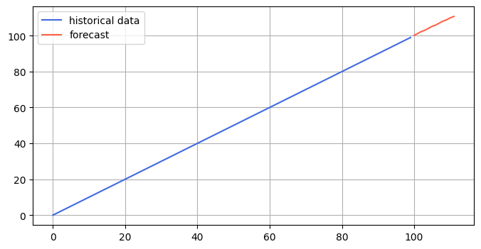
As you can see, the model is performing as expected. You can note that the predictions are not integers in the forecast but rather float. This is expected as the model typically operates on float values and needs help forecasting exact integers.
You should note that on the GitHub page, the predict function is given with num_samples=20, which will return 20 predictions for the predicted time series. The minimum, median, and maximum predictions can be visualized using the visualization code on the GitHub page. I, however, chose to keep the code as simple as possible and only use num_samples=1.
Tasks you can use the model for
There are numerous tasks for which you can use this model. Considering it is a traditional time-series forecasting model, you can use it for any time you want to predict future values, given past values. Classic examples of tasks where this is the case are:
- Energy usage
- Weather
- Traffic prediction
- And much more
Another interesting use case is taking the embeddings the model gives you. Embeddings are very useful overall within machine learning, something I have written about in more detail in my Towards Data Science article below:
For example, you can use the embeddings from the Chronos time series forecasting model to cluster different time series. Given an embedding of many time series, you can cluster the different time series close to each other based on the similarity between the embeddings. Another exciting use case of time series embeddings is to train an LLM to explain the time series given by time series embedding. With this, you can have the model explain the time series and potentially use the Chronos predictions to the LLM to provide the LLM with access to future predictions.
All in all, a time series model has countless applications, and it can generally be applied to any time series prediction task.
Dataset
I am using some publicly available time-series datasets to test how the model performs. I found this GitHub page [3] that gives easy access to 169 different time-series datasets, which I will utilize. The data follows a BSD-3 license, shown at the bottom of this article.
The first dataset I am using is the physionet_2012 dataset [3], which you can load with:
import tsdb
data = tsdb.load('physionet_2012')
This will then load a dataframe with several columns you can use. I am using the Temp column:
timeseries = data["X"]["Temp"].to_numpy()
#remove nan values
physionet_2012_timeseries = timeseries[~np.isnan(timeseries)]
You should note that the dataset has many NaN values, which I removed with the code above.
Accuracy measurements
I use three different accuracy measurements to calculate the performance of the time series forecasting:
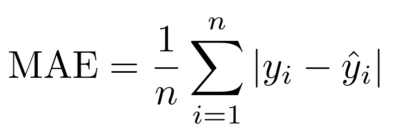
- MAE — Mean absolute error
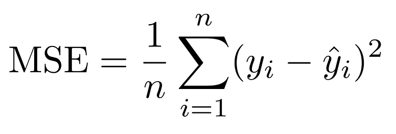
- MSE — Mean squared error
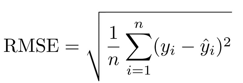
- RMSE — Root mean squared error
Mean absolute error is a useful measurement since it gives an error estimate that is easy for the human mind to interpret. Say, for example, I am predicting temperatures. If the mean absolute error of the time series forecasting model for temperature is 4, I know the temperature is, on average, off by two degrees. You can then consider this error number to determine if the model performs well or poorly. In this case, missing the temperature by four degrees on average is quite bad, and the model performs poorly.
The mean squared error can be more difficult to interpret directly, as you can with the mean absolute error. The idea behind squaring the error is that you punish more significant errors than minor ones. The reason why more significant errors are punished more than minor ones can be understood by the following example. Say model A has an average error of 2, and model B has an average of 4. Model A is twice as good as model B in terms of mean absolute error. If we look at the mean squared error, however, model A will have a squared error of 4, and model B will have a squared error of 16. In terms of squared error, model A is four times better than model B. Thus, more significant errors are punished more than minor errors.
If it is difficult to be sure which error you should use, different metrics will be better in various scenarios. However, calculating the MAE, MSE, and RMSE a cheap operations. Thus, you can perform all three computations in a short amount of time. You can then look at all three metrics to determine the model's performance. Though it is more difficult to understand the meaning of a mean squared error, you can compare the error relative to other models and, in that way, understand how well a model performs.
The root mean squared error is the root of the squared error. This metric can be seen as a middle ground between the mean absolute error and the mean squared error. The mean absolute error is interpretable because you are taking the root of a squared number, which is the number itself. However, you also get the effect of punishing larger errors more since you are squaring the number before taking the root.
During my model testing, all three metrics were used to understand how well the model performs. To calculate the scores with Python, I use the following code:
def get_mse(y_true, y_pred):
 return np.mean((y_true - y_pred)**2)
def get_mae(y_true, y_pred):
 return np.mean(np.abs(y_true - y_pred))
def get_rmse(y_true, y_pred):
 return np.sqrt(get_mse(y_true, y_pred))

def get_scores(y_true, y_pred):
 """given true and predicted values, return mse, mae, rmse"""
 return get_mse(y_true, y_pred), get_mae(y_true, y_pred), get_rmse(y_true, y_pred)
Having relevant metrics to measure model performance is vital to ensure model testing is done correctly. You can learn more about testing within machine learning in my article below:
Testing the model
I can then test the model. First, I use the physionet_2012 dataset, which you can load and pre-process with:
pipeline = load_model()
data = tsdb.load('physionet_2012')
timeseries = data["X"]["Temp"].to_numpy()
physionet_2012_timeseries = timeseries[~np.isnan(timeseries)]
Then, to test the model, I give the model a context window and ask it to predict the following values given that context window. I then ensure that the ground truth values are also included in the values I forecast so the error can be calculated with MAE, MSE, and RMSE. You can do this with the following code:
# now test the model. Given the last x values, predict the next y values, then we can calculate metrics like MSE, RMSE, MAE
CONTEXT_LENGTH = 100
PREDICTION_LENGTH = 10


mse_scores, mae_scores, rmse_scores = [], [], []
for i in tqdm(range(0, len(physionet_2012_timeseries), CONTEXT_LENGTH)):
 if (i+CONTEXT_LENGTH+PREDICTION_LENGTH) > len(physionet_2012_timeseries):
  break
 prediction = predict(pipeline, torch.tensor(physionet_2012_timeseries[i:i+CONTEXT_LENGTH]), PREDICTION_LENGTH)
 ground_truth = physionet_2012_timeseries[i+CONTEXT_LENGTH:i+CONTEXT_LENGTH+PREDICTION_LENGTH]

 mse, mae, rmse = get_scores(ground_truth, prediction.numpy())
 mse_scores.append(mse), mae_scores.append(mae), rmse_scores.append(rmse)
With context length set to 100 and prediction length set to 10, I get the following results:
MAE:   1.15
MSE:   54.78
RMSE:  1.57
So, on average, the model misses with an absolute error of 1.28, which I consider a decent performance in the context of temperatures.
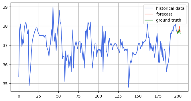
The model should, however, perform better with an increased context length and shorter prediction length. I test this by setting CONTEXT_LENGTH=200, and PREDICTION_LENGTH=5, and get the following results:
MAE:   0.85
MSE:   2.21
RMSE:  1.01
As you can see, the model performs quite a bit better!
You can see a plot below showing the forecasting of the model compared to the ground truth:
To make the forecasting vs ground truth more evident, you can zoom in on the forecasted y values:
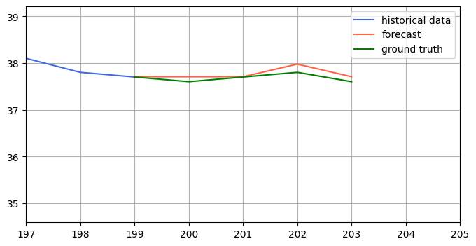
My thoughts on the model
First of all, the model was very simple to set up. Everything in the README worked as expected, and I got the model working right away. Furthermore, the model is also simple to use. All you need to do is put it in a one-dimensional array, specify the number of steps you want to be forecasted, and the model takes care of the rest. The authors also included an easy way to visualize the time series and the prediction. Furthermore, code was provided in GitHub to access the embeddings of the model if that is of interest.
Testing the model also proves that it performs well. I ran the model on a publicly available dataset consisting of temperatures. With a context window of 200 and making predictions 5 steps into the future, the model performs with a mean absolute error well under 1. This decent performance proves the model is worthwhile looking into if you are currently working on a time series forecasting problem.
Naturally, this is only surface-level testing of the model, but I think surface-level testing can still give valuable insight into whether or not you should use it. The model definitely has good potential, though how well it performs for your use case will depend on the circumstances.
Future work
This is only a short introduction and experimentation of the Chronos time series forecasting model. There is much more I would like to do to further test out the model:
- Try out the embeddings from the model to see how I can utilize them. For example, performing clustering on time series
- Compare the model performance against other State-of-the-Art time series forecasting models
- Try the model out actively to predict energy usage. You can, for example, do this by gathering live data on energy usage in an area and storing the forecasted values. After you can see the true energy usage, you can find the accuracy of the model.
Conclusion
This article discusses Amazon's new time series forecasting model. I have discussed some tasks the model can be applied to and how you can run the model locally in Python. Furthermore, I downloaded a publicly available dataset to test the model's performance and discussed my thoughts on the model.
You can check out the complete code on my GitHub.
You can also read my articles on WordPress.
The package I got the data from follows a BSD-3-Clause license:
Copyright (c) 2023-present, Wenjie Du
All rights reserved.

Redistribution and use in source and binary forms, with or without
modification, are permitted provided that the following conditions are met:

1. Redistributions of source code must retain the above copyright
   notice, this list of conditions and the following disclaimer.

2. Redistributions in binary form must reproduce the above copyright
   notice, this list of conditions and the following disclaimer in the
   documentation and/or other materials provided with the distribution.

3. Neither the name of the copyright holder nor the names of its
   contributors may be used to endorse or promote products derived from
   this software without specific prior written permission.

THIS SOFTWARE IS PROVIDED BY THE COPYRIGHT HOLDERS AND CONTRIBUTORS "AS IS"
AND ANY EXPRESS OR IMPLIED WARRANTIES, INCLUDING, BUT NOT LIMITED TO, THE
IMPLIED WARRANTIES OF MERCHANTABILITY AND FITNESS FOR A PARTICULAR PURPOSE
ARE DISCLAIMED. IN NO EVENT SHALL THE COPYRIGHT OWNER OR CONTRIBUTORS BE
LIABLE FOR ANY DIRECT, INDIRECT, INCIDENTAL, SPECIAL, EXEMPLARY, OR
CONSEQUENTIAL DAMAGES (INCLUDING, BUT NOT LIMITED TO, PROCUREMENT OF
SUBSTITUTE GOODS OR SERVICES; LOSS OF USE, DATA, OR PROFITS; OR BUSINESS
INTERRUPTION) HOWEVER CAUSED AND ON ANY THEORY OF LIABILITY, WHETHER IN
CONTRACT, STRICT LIABILITY, OR TORT (INCLUDING NEGLIGENCE OR OTHERWISE)
ARISING IN ANY WAY OUT OF THE USE OF THIS SOFTWARE, EVEN IF ADVISED OF THE
POSSIBILITY OF SUCH DAMAGE.
References
[1] Ansari, A. F., Stella, L., Turkmen, C., Zhang, X., Mercado, P., Shen, H., Shchur, O., Rangapuram, S. S., Pineda Arango, S., Kapoor, S., Zschiegner, J., Maddix, D. C., Mahoney, M. W., Torkkola, K., Wilson, A. G., Bohlke-Schneider, M., & Wang, Y. (2024). Chronos: Learning the language of time series. arXiv preprint arXiv:2403.07815.
[2] Du, W. (2023). PyPOTS: A Python toolbox for data mining on Partially-Observed Time Series. arXiv preprint arXiv:2305.18811. https://doi.org/10.48550/arXiv.2305.18811
[3] Silva I, Moody G, Scott DJ, Celi LA, Mark RG. Predicting In-Hospital Mortality of ICU Patients: The PhysioNet/Computing in Cardiology Challenge 2012. Comput Cardiol (2010). 2012;39:245–248. PMID: 24678516; PMCID: PMC3965265.


