How to Draw a Map using Python and Word2vec

A 2-D visual representation of the principal components created from the Word2vec vectors of European capitals — a.k.a. a map.

Word2vec is definitely the most playful concept I’ve met during my Natural Language Processing studies so far. Imagine an algorithm that can really successfully mimic understanding meanings of words and their functions in the language, that can measure the closeness of words along the lines of hundreds of different topics, that can answer more complicated questions like “who was to literature what Beethoven was to music”.

I thought it would be interesting to visually represent word2vec vectors: essentially, we can take the vectors of countries or cities, apply principal component analysis to reduce the dimensions, and put them on a 2-D chart. And then, we can observe how close we are to an actual geographical map.

In this post, we are going to:

• discuss the word2vec theory in broad terms;
• download the original pre-trained vectors;
• check out a few playful applications: finding the odd one out of a list or doing arithmetical operations on words like the famous king — man + woman = queen example;
• see how accurately we can draw the capitals of Europe based on nothing else but the word2vec vectors.

The original word2vec research paper and the pre-trained model is from 2013, and considering the rate with which the NLP literature is expanding, it’s old technology at this point. Newer approaches include GloVe (faster training, different algorithm, can be trained on smaller corpus) and fastText (capable of handling character n-grams). I’m sticking with the results of the original algorithm for now.

Quick Word2Vec Intro

One of the core concepts of Natural Language Processing is how we can quantify words and expressions in order to be able to work with them in a model setting. This mapping of language elements to numerical representations is called word embedding.

Word2vec is a word embedding process. The concept is relatively simple: sentence by sentence, it loops through the corpus, and fits a model that predicts words based on neighbouring words from a pre-defined sized window. To do that, it uses a neural network, but doesn’t actually use the predictions, once the model is saved, it only saves the weights from the first layer. In the original model, the one we are going to use, there are 300 weights, so every word is represented by a 300-dimensional vector.

Note that two words don’t have to be in each other’s proximity to be deemed similar. If two words never appear in the same sentence, but they are usually surrounded by the same words, it is safe to assume that they have a similar meaning.

There are two modelling approaches within word2vec: skip-gram and continuous bag-of-words, both with their own advantages and sensitivities to certain hyperparameters… but you know what? We aren’t going to fit our own model, so I’m not going to spend more time on it, you can read more about the different approaches and parameters in this article or the wiki site.

Naturally, the word vectors you get depend on the corpus you train your model on. Generally, you do need a huge corpus, there are versions trained on Wikipedia, or news articles from various sources. The results that we are going to use were trained on Google News.

How to Download & Install

First, you will need to download pre-trained word2vec vectors. You can choose from a wide variety of models, trained on different types of documents. I went with the original model, trained on Google News, which you can download from many sources, just search for “Google News vectors negative 300”. For example, this GitHub link is a convenient method: https://github.com/mmihaltz/word2vec-GoogleNews-vectors.

Be careful, the file is 1.66 GB, but in its defence, it contains the 300-dimensional representation of 3 billion words.

When it comes to working with word2vec in Python, once again, you have a lot of packages to choose from, we are going to use the gensim library. Assuming you have the file saved in the word2vec_pretrained folder, you can load it in Python like so:

from gensim.models.keyedvectors import KeyedVectors

word_vectors = KeyedVectors.load_word2vec_format(\
    './word2vec_pretrained/GoogleNews-vectors-negative300.bin.gz', \
    binary = True, limit = 1000000)

The limit parameter defines how many words you are importing, 1 million was plenty enough for my purposes.

Playing with Words

Now that we have the word2vec vectors in place, we can check out some of its applications.

First of all, you can actually check the vector representation of any word:

word_vectors['dog']

The result is, as we expected, a 300-dimensional vector that is quite difficult to interpret. But that’s the basis of the whole concept, we are making calculations on these vectors by adding and subtracting them from each other, and then we calculate the cosine similarities to find closest matching words.

You can find synonyms with the most_similar function, the topn parameter defines how many words you want to be listed:

word_vectors.most_similar(positive = ['nice'], topn = 5)

results in

[('good', 0.6836092472076416),
 ('lovely', 0.6676311492919922),
 ('neat', 0.6616737246513367),
 ('fantastic', 0.6569241285324097),
 ('wonderful', 0.6561347246170044)]

Now, you might think that with a similar approach, you can also find antonyms, you just need to enter the word ‘nice’ as a negative, right? Not really, the result is this:

[('J.Gordon_###-###', 0.38660115003585815),
 ('M.Kenseth_###-###', 0.35581791400909424),
 ('D.Earnhardt_Jr._###-###', 0.34227001667022705),
 ('G.Biffle_###-###', 0.3420777916908264),
 ('HuMax_TAC_TM', 0.3141660690307617)]

These are the words that are farthest away from the word ‘nice’, suggesting that it does not always work as you would expect.

You can find odd ones out using the doesnt_match function:

word_vectors.doesnt_match(
['Hitler', 'Churchill', 'Stalin', 'Beethoven'])

returns Beethoven. Which is handy, I guess.

And finally, let’s see a couple of examples of the operations that made the algorithm famous by giving it a false sense of intelligence. If we want to combine the values of the word vectorsfather and woman but subtract the values assigned to the word vectorman:

word_vectors.most_similar(
positive = ['father', 'woman'], negative = ['man'], topn = 1)

we get:

[('mother', 0.8462507128715515)]

It’s a bit difficult to wrap your head around this operation first, and I think phrasing the question like “What is to a woman that father is to a man?” is not really that helpful. Imagine that we have only 2 dimensions: parentness and gender. The word ‘woman’ might be represented by this vector: [0, 1], ‘man’ is[0, -1], ‘father’ would be [1, -1], and ‘mother’ would be [1, 1]. Now, if we do the same operations as we did up there with the word vectors, we get the same results. Of course, the difference is that we have 300 dimensions instead of the mere 2 in the example, and the dimensions’ meaning are nigh impossible to interpret.

There was a famous example of gender bias when it came to word2vec operations, the woman version of the word ‘doctor’ (which is, as we know, a gender-neutral word) used to be calculated as ‘nurse’. I tried replicating it, but did not get the same result:

word_vectors.most_similar(
positive = ['doctor', 'woman'], negative = ['man'], topn = 1)

[('gynecologist', 0.7093892097473145)]

So, progress, I guess?

All right, now that we checked out a few of the basic possibilities, let’s work on our map!

Mapping Function

First, we need a plan of what we want our mapping function to do. Assuming we have a list of strings we want to visualise and a word vector object, we want to:

1. find the word vector representation of each word in the list;
2. reduce the dimensions to 2 using principal component analysis;
3. create a scatter plot, add the words as labels to each data point;
4. as an added bonus, make it possible to “flip” the results by any dimension — the vectors from the principal component analysis are of an arbitrary direction, which we might want to change when we plot geographical words to better align with the real-world directions.

We will need the following libraries:

import matplotlib.pyplot as plt
import seaborn as sns
from sklearn.decomposition import PCA

import adjustText

One library that is not commonly used from the list is adjustText, it’s a very handy package that makes it simple to write legends in scatter plots, without them overlapping. It was surprisingly hard for me to find this solution, and as far as I know, there is no way to do this in matplotlib or seaborn.

Without further ado, this is the function that will do exactly what we need:

def plot_2d_representation_of_words(
    word_list, 
    word_vectors, 
    flip_x_axis = False,
    flip_y_axis = False,
    label_x_axis = "x",
    label_y_axis = "y", 
    label_label = "city"):
    
    pca = PCA(n_components = 2)
    
    word_plus_coordinates=[]
    
    for word in word_list: 
    
        current_row = []
        current_row.append(word)
        current_row.extend(word_vectors[word])

    word_plus_coordinates.append(current_row)
    
    word_plus_coordinates = pd.DataFrame(word_plus_coordinates)
        
    coordinates_2d = pca.fit_transform(
        word_plus_coordinates.iloc[:,1:300])
    coordinates_2d = pd.DataFrame(
        coordinates_2d, columns=[label_x_axis, label_y_axis])
    coordinates_2d[label_label] = word_plus_coordinates.iloc[:,0]

    if flip_x_axis:
        coordinates_2d[label_x_axis] = \
        coordinates_2d[label_x_axis] * (-1)

    if flip_y_axis:
        coordinates_2d[label_y_axis] = \
        coordinates_2d[label_y_axis] * (-1)
            
    plt.figure(figsize = (15,10))

    p1=sns.scatterplot(
        data=coordinates_2d, x=label_x_axis, y=label_y_axis)
    
    x = coordinates_2d[label_x_axis]
    y = coordinates_2d[label_y_axis]
    label = coordinates_2d[label_label]
    
    texts = [plt.text(x[i], y[i], label[i]) for i in range(len(x))]

    adjustText.adjust_text(texts)

Now it’s time to test the function. I plotted the capitals of the European countries, but you can use literally any list, names of presidents or other historical figures, car brands, cooking ingredients, rock bands, etc, just pass it in the word_list parameter. I had some fun with it, it’s interesting to see clusters forming up and trying to come up with a meaning behind the two axes.

In case you want to reproduce the results, here are the cities:

capitals = [
    'Amsterdam', 'Athens', 'Belgrade', 'Berlin', 'Bern', 
    'Bratislava', 'Brussels', 'Bucharest', 'Budapest', 
    'Chisinau', 'Copenhagen','Dublin', 'Helsinki', 'Kiev',
    'Lisbon', 'Ljubljana', 'London', 'Luxembourg','Madrid',
    'Minsk', 'Monaco', 'Moscow', 'Nicosia', 'Nuuk', 'Oslo', 
    'Paris','Podgorica', 'Prague', 'Reykjavik', 'Riga', 
    'Rome', 'San_Marino', 'Sarajevo','Skopje', 'Sofia', 
    'Stockholm', 'Tallinn', 'Tirana', 'Vaduz', 'Valletta',
    'Vatican', 'Vienna', 'Vilnius', 'Warsaw', 'Zagreb']

(Andorra’s capital, Andorra la Vella is missing from the list, couldn’t find a format that word2vec recognises. We will live with that.)

Assuming you still have the word_vectors object we created in the previous section, you can call the function like so:

plot_2d_representation_of_words(
    word_list = capitals, 
    word_vectors = word_vectors, 
    flip_y_axis = True)

(Axis y is flipped in order to create a representation that better resembles a real map.)

And the result is:

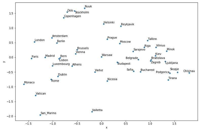
I don’t know how you feel, when I first saw the map, I couldn’t believe how well it turned out! Yes, sure, the longer you look, the more “mistakes” you find, one ominous outcome is that Moscow is not as far to the east as it should be… Still, east and west are almost perfectly separated, Scandinavian and Baltic countries are nicely grouped, so are capitals around Italy, and the list goes on.

It’s important to emphasise that this was never meant to be purely the geographical location, for example, Athens is very far to the west, but there’s a reason for that. Let’s recap how the map above is derived, just so we can fully appreciate it:

• a group of researchers at Google trained a gigantic neural network that predicted words based on their context;
• they saved the weights of every single word in a 300-dimensional vector representation;
• we took the vectors of the European capitals;
• reduced the dimensions to 2 by using principal component analysis;
• put the calculated components on a chart.

And I think that’s pretty awesome!

References

Hobson, L. & Cole, H. & Hannes, H. (2019). Natural Language Processing in Action: Understanding, Analyzing, and Generating Text with Python. Manning Publications, 2019.