avatarBen Hui

Free AI web copilot to create summaries, insights and extended knowledge, download it at here

3050

Abstract

n>, <span class="hljs-number">1200</span>, <span class="hljs-number">1400</span>, <span class="hljs-number">1600</span>, <span class="hljs-number">1800</span>, <span class="hljs-number">2000</span>, <span class="hljs-number">2200</span>, <span class="hljs-number">2400</span>], [<span class="hljs-number">1200</span>, <span class="hljs-number">1400</span>, <span class="hljs-number">1600</span>, <span class="hljs-number">1800</span>, <span class="hljs-number">2000</span>, <span class="hljs-number">2200</span>, <span class="hljs-number">2400</span>, <span class="hljs-number">2600</span>], [<span class="hljs-number">1400</span>, <span class="hljs-number">1600</span>, <span class="hljs-number">1800</span>, <span class="hljs-number">2000</span>, <span class="hljs-number">2200</span>, <span class="hljs-number">2400</span>, <span class="hljs-number">2600</span>, <span class="hljs-number">2800</span>], [<span class="hljs-number">1600</span>, <span class="hljs-number">1800</span>, <span class="hljs-number">2000</span>, <span class="hljs-number">2200</span>, <span class="hljs-number">2400</span>, <span class="hljs-number">2600</span>, <span class="hljs-number">2800</span>, <span class="hljs-number">3000</span>], [<span class="hljs-number">1800</span>, <span class="hljs-number">2000</span>, <span class="hljs-number">2200</span>, <span class="hljs-number">2400</span>, <span class="hljs-number">2600</span>, <span class="hljs-number">2800</span>, <span class="hljs-number">3000</span>, <span class="hljs-number">3200</span>], [<span class="hljs-number">2000</span>, <span class="hljs-number">2200</span>, <span class="hljs-number">2400</span>, <span class="hljs-number">2600</span>, <span class="hljs-number">2800</span>, <span class="hljs-number">3000</span>, <span class="hljs-number">3200</span>, <span class="hljs-number">3400</span>], [<span class="hljs-number">2200</span>, <span class="hljs-number">2400</span>, <span class="hljs-number">2600</span>, <span class="hljs-number">2800</span>, <span class="hljs-number">3000</span>, <span class="hljs-number">3200</span>, <span class="hljs-number">3400</span>, <span class="hljs-number">3600</span>], [<span class="hljs-number">2400</span>, <span class="hljs-number">2600</span>, <span class="hljs-number">2800</span>, <span class="hljs-number">3000</span>, <span class="hljs-number">3200</span>, <span class="hljs-number">3400</span>, <span class="hljs-number">3600</span>, <span class="hljs-number">3800</span>] ])

fig = plt.figure() ax = fig.add_subplot(<span class="hljs-number">111</span>, projection=<span class="hljs-string">'3d'</span>)

ax.plot_surface(price, sale, performance, cmap=<span class="hljs-string">'coolwarm'</span>)

ax.set_xlabel(<span class="hljs-string">'Price'</span>) ax.set_ylabel(<span class="hljs-string">'Sales'</span>) ax.set_zlabel(<span class="hljs-string">'Performance'</span>)

ax.set_title(<span class="hljs-string">'Sales Performance with Price and Sales'</span>)

plt.show()</pre></div><figure id="b92a"><img src="https://

Options

cdn-images-1.readmedium.com/v2/resize:fit:800/1*4OmTRtq6QQ5y2x7i1cFZHg.png"><figcaption></figcaption></figure><p id="7ae5">Here performance is a 2D array. Every cell of it means a performance with corresponding price and sales. In this case, higher surface means higher performance. So we can find a best price-sales point.</p><p id="3588">Sometimes, we may need multiple plots displaying in the mean time:</p><div id="fbdd"><pre><span class="hljs-keyword">import</span> numpy <span class="hljs-keyword">as</span> np <span class="hljs-keyword">import</span> matplotlib.pyplot <span class="hljs-keyword">as</span> plt <span class="hljs-keyword">from</span> mpl_toolkits.mplot3d <span class="hljs-keyword">import</span> Axes3D

x = np.linspace(-<span class="hljs-number">5</span>, <span class="hljs-number">5</span>, <span class="hljs-number">100</span>) y = np.linspace(-<span class="hljs-number">5</span>, <span class="hljs-number">5</span>, <span class="hljs-number">100</span>) X, Y = np.meshgrid(x, y) Z1 = np.sin(np.sqrt(X**<span class="hljs-number">2</span> + Y**<span class="hljs-number">2</span>)) Z2 = np.cos(X) * np.sin(Y) Z3 = np.exp(-(X**<span class="hljs-number">2</span> + Y**<span class="hljs-number">2</span>)/<span class="hljs-number">10</span>) * np.cos(np.sqrt(X**<span class="hljs-number">2</span> + Y**<span class="hljs-number">2</span>))

fig = plt.figure()

<span class="hljs-comment"># plog 1</span> ax1 = fig.add_subplot(<span class="hljs-number">131</span>, projection=<span class="hljs-string">'3d'</span>) ax1.plot_surface(X, Y, Z1, cmap=<span class="hljs-string">'viridis'</span>) ax1.set_xlabel(<span class="hljs-string">'X'</span>) ax1.set_ylabel(<span class="hljs-string">'Y'</span>) ax1.set_zlabel(<span class="hljs-string">'Z1'</span>)

<span class="hljs-comment"># plog 2</span> ax2 = fig.add_subplot(<span class="hljs-number">132</span>, projection=<span class="hljs-string">'3d'</span>) ax2.plot_surface(X, Y, Z2, cmap=<span class="hljs-string">'plasma'</span>) ax2.set_xlabel(<span class="hljs-string">'X'</span>) ax2.set_ylabel(<span class="hljs-string">'Y'</span>) ax2.set_zlabel(<span class="hljs-string">'Z2'</span>)

<span class="hljs-comment"># plot 3</span> ax3 = fig.add_subplot(<span class="hljs-number">133</span>, projection=<span class="hljs-string">'3d'</span>) ax3.plot_surface(X, Y, Z3, cmap=<span class="hljs-string">'magma'</span>) ax3.set_xlabel(<span class="hljs-string">'X'</span>) ax3.set_ylabel(<span class="hljs-string">'Y'</span>) ax3.set_zlabel(<span class="hljs-string">'Z3'</span>)

fig.suptitle(<span class="hljs-string">'Multiple 3D Surface Plots'</span>)

fig.tight_layout()

plt.show()</pre></div><figure id="db69"><img src="https://cdn-images-1.readmedium.com/v2/resize:fit:800/1*jelP7p2bdnacJG7lJpWcmg.png"><figcaption></figcaption></figure><p id="649e">Like 2D plots, use “add_subplot” to create a 1*3 figure here. Then draw the plot for specific position. “tight_layout()” is able to make the whole figure more visible.</p><p id="ad77">Thank you for reading.</p></article></body>

How to draw 3D surface plots in Python

A 3D surface plot is usually used for the data with 1 dependent variable and 2 independent variables. It can display the trend, shape and spatial distribution. In this article, I am going to introduce how to use Python code to draw 3D surface plots.

Let’s see a basic one first:

import numpy as np
import matplotlib.pyplot as plt
from mpl_toolkits.mplot3d import Axes3D

x = np.linspace(-5, 5, 100)
y = np.linspace(-5, 5, 100)
X, Y = np.meshgrid(x, y)
Z = np.sin(np.sqrt(X**2 + Y**2))

fig = plt.figure()
ax = fig.add_subplot(111, projection='3d')

ax.plot_surface(X, Y, Z, cmap='viridis')

ax.set_xlabel('X')
ax.set_ylabel('Y')
ax.set_zlabel('Z')

ax.set_title('3D Surface Plot')

plt.show()

Assuming that we have some sales data. It contains prices and sales. We can use a 3D surface plot to visual the data to display the relationship of prices and sales:

import numpy as np
import matplotlib.pyplot as plt
from mpl_toolkits.mplot3d import Axes3D

# Price
prices = np.array([10, 20, 30, 40, 50, 60, 70, 80])
# Sales
sales = np.array([100, 150, 200, 250, 300, 350, 400, 450])

price, sale = np.meshgrid(prices, sales)

# Performance
performance = np.array([
    [1000, 1200, 1400, 1600, 1800, 2000, 2200, 2400],
    [1200, 1400, 1600, 1800, 2000, 2200, 2400, 2600],
    [1400, 1600, 1800, 2000, 2200, 2400, 2600, 2800],
    [1600, 1800, 2000, 2200, 2400, 2600, 2800, 3000],
    [1800, 2000, 2200, 2400, 2600, 2800, 3000, 3200],
    [2000, 2200, 2400, 2600, 2800, 3000, 3200, 3400],
    [2200, 2400, 2600, 2800, 3000, 3200, 3400, 3600],
    [2400, 2600, 2800, 3000, 3200, 3400, 3600, 3800]
])

fig = plt.figure()
ax = fig.add_subplot(111, projection='3d')

ax.plot_surface(price, sale, performance, cmap='coolwarm')

ax.set_xlabel('Price')
ax.set_ylabel('Sales')
ax.set_zlabel('Performance')

ax.set_title('Sales Performance with Price and Sales')

plt.show()

Here performance is a 2D array. Every cell of it means a performance with corresponding price and sales. In this case, higher surface means higher performance. So we can find a best price-sales point.

Sometimes, we may need multiple plots displaying in the mean time:

import numpy as np
import matplotlib.pyplot as plt
from mpl_toolkits.mplot3d import Axes3D

x = np.linspace(-5, 5, 100)
y = np.linspace(-5, 5, 100)
X, Y = np.meshgrid(x, y)
Z1 = np.sin(np.sqrt(X**2 + Y**2))
Z2 = np.cos(X) * np.sin(Y)
Z3 = np.exp(-(X**2 + Y**2)/10) * np.cos(np.sqrt(X**2 + Y**2))

fig = plt.figure()

# plog 1
ax1 = fig.add_subplot(131, projection='3d')
ax1.plot_surface(X, Y, Z1, cmap='viridis')
ax1.set_xlabel('X')
ax1.set_ylabel('Y')
ax1.set_zlabel('Z1')

# plog 2
ax2 = fig.add_subplot(132, projection='3d')
ax2.plot_surface(X, Y, Z2, cmap='plasma')
ax2.set_xlabel('X')
ax2.set_ylabel('Y')
ax2.set_zlabel('Z2')

# plot 3
ax3 = fig.add_subplot(133, projection='3d')
ax3.plot_surface(X, Y, Z3, cmap='magma')
ax3.set_xlabel('X')
ax3.set_ylabel('Y')
ax3.set_zlabel('Z3')

fig.suptitle('Multiple 3D Surface Plots')

fig.tight_layout()

plt.show()
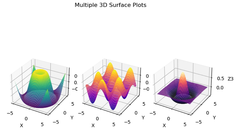
Like 2D plots, use “add_subplot” to create a 1*3 figure here. Then draw the plot for specific position. “tight_layout()” is able to make the whole figure more visible.

Thank you for reading.

Python
Data Science
Data Analysis
Data Visualization
Data
Recommended from ReadMedium