
How to Download Sentinel-2 Images in R (Updated January 2024)
In this story, I’ll guide you through the process of downloading Sentinel-2 images in R using the recently introduced API structure available at https://dataspace.copernicus.eu/.
Table of Contents
- 🌟 Introduction
- 🔍 Install and Import the Libraries
- ⏳ Filter and Submit the Query
- 🔐 Create the Access Token
- 📥 Download the Metadata File (.xml)
- 📜 Read the Metadata File and Extract URL Path
- 📥 Download the “jp2” files
- 🛠️ Read the “jp2” files, Stack, and Clip it to AOI
- 📈 Plot the True Color of the Surface Reflectance Images
- 📚 References
🌟 Introduction
In July 2023, I published my first story on Medium, detailing the process of downloading Sentinel-2 images using R. Over time, this story gained many reads and became my most viewed article. However, a new API structure was introduced two or three months later, and obviously, the R script of that article was not useful anymore. Therefore, I wrote a new article on downloading Sentinel-2 images in Python in December 2023, which now holds the top spot in my list of most-viewed articles.
Realizing that many users might still be working with R for satellite image downloads, I wanted to update my original article. However, the first article still has valuable sections on adding satellite base maps to QGIS, drawing polygons, and saving them as shapefiles for use in scripts. To keep this content, I decided to leave the initial article unchanged and instead write a fresh one on downloading Sentinel-2 images in R with the updated date in the title.
I won’t repeat the steps for signing up on the new website and creating credentials, as I’ve described those steps in this post:
Instead, I’ll be focusing on converting the script I wrote in Python (Google Colab) to a script in R (R-studio). I hope you find this approach useful and enjoy these steps to download Sentinel-2 images for your AOI.
🔍 Install and Import the Libraries
Let’s start by installing these libraries if they haven’t been installed on your system yet:
# Install necessary packages if not already installed
install.packages("httr")
install.packages("jsonlite")
install.packages("dplyr")
install.packages("xml2")
install.packages("raster")
install.packages("sf")
and load them into the memory:
# Load required libraries
library(httr)
library(jsonlite)
library(dplyr)
library(xml2)
library(raster)
library(sf)
⏳ Filter and Submit the Query
To gain access to metadata and filter images based on dates and location, you don’t need to use your credentials. In this step, you only need to input the database URL and provide the required information, such as satellite name, product level (e.g., “S2MI2A” for surface reflectance), and the area of interest:
# Define the base URL for the Copernicus Data Space API
url_dataspace <- "https://catalogue.dataspace.copernicus.eu/odata/v1"

# Define filtering parameters
satellite <- "SENTINEL-2"
level <- "S2MSI2A"
cloud_cover_max <- 1

# Define Area of Interest (AOI) in point or polygon formats
#aoi_point <- "POINT(-120.9970 37.6393)"
aoi_polygon <- "POLYGON ((-121.0616 37.6391, -120.966 37.6391, -120.966 37.6987, -121.0616 37.6987, -121.0616 37.6391))"

# Define start and end dates for data acquisition
start_date <- "2023-11-01"
end_date <- "2023-11-10"
start_date_full <- paste0(start_date, "T00:00:00.000Z")
end_date_full <- paste0(end_date, "T00:00:00.000Z")
Next, pass the URL and that information to the query command to obtain the results:
# Construct the query to filter products based on specified parameters
query <- paste0(url_dataspace, "/Products?$filter=Collection/Name%20eq%20'", satellite, "'%20and%20Attributes/OData.CSC.StringAttribute/any(att:att/Name%20eq%20'productType'%20and%20att/OData.CSC.StringAttribute/Value%20eq%20'", level, "')%20and%20OData.CSC.Intersects(area=geography'SRID=4326;", URLencode(aoi_point), "')%20and%20ContentDate/Start%20gt%20", start_date_full, "%20and%20ContentDate/Start%20lt%20", end_date_full)
response <- GET(query)
The response will be a JSON file that needs to be converted to a dataframe. Next, we will filter the records that are “online” and available on the database server:
# Extract and process the JSON response
response_content <- content(response, "text", encoding = "UTF-8")
response_json <- fromJSON(response_content)
result <- as.data.frame(response_json$value)

# Filter records where 'Online' column is TRUE
result <- filter(result, Online == TRUE)

# Display the first 10 results
head(result, 10)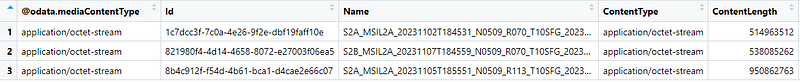
🔐 Create the Access Token
After obtaining a list of available images in the dataframe format, we can use our credentials to generate a token, which can later be used for downloading the image:
# Authentication for accessing secured resources
username = "Your Username"
password = "Your Password"

# Define authentication server URL
auth_server_url <- "https://identity.dataspace.copernicus.eu/auth/realms/CDSE/protocol/openid-connect/token"

# Prepare authentication data
data <- list(
  "client_id" = "cdse-public",
  "grant_type" = "password",
  "username" = username,
  "password" = password
)

# Request access token
response <- POST(auth_server_url, body = data, encode = "form", verify = TRUE)
access_token <- fromJSON(content(response, "text", encoding = "UTF-8"))$access_token
📥 Download the metadata file (.xml)
After generating the token, the next step is to extract the complete URL path generated for each band from the metadata. Each image listed in the dataframe has its own metadata. In this article, the focus is on processing the third image in the list captured on Nov 5th, 2023 around 18:00 UTM. (S2A_MSIL2A_20231105T185551_N0509_R113_T10SFG_20231105T222401):
# Set the Authorization header using obtained access token
headers <- add_headers(Authorization = paste("Bearer", access_token))

# Extract product information for the third product in the list
product_row_id <- 3 # The third images in the list (Nov 5th, 2023)
product_id <- result[product_row_id, "Id"]
product_name <- result[product_row_id, "Name"]

# Create the URL for MTD file
url_MTD <- paste0(url_dataspace, "/Products(", product_id, ")/Nodes(", product_name, ")/Nodes(MTD_MSIL2A.xml)/$value")

# GET request for MTD file and handle redirects
response <- httr::GET(url_MTD, headers, config = httr::config(followlocation = FALSE))
print(response$status_code)

# Extract the final URL for MTD file
url_MTD_location <- response$headers[["Location"]]
print(url_MTD_location)

# Download the MTD file
file <- httr::GET(url_MTD_location, headers, config = httr::config(ssl_verifypeer = FALSE, followlocation = TRUE))

# Set working directory and save the MTD file
setwd("C:/Users/Project/Sentinel-2")
outfile <- file.path(getwd(), "MTD_MSIL2A.xml")
writeBin(content(file, "raw"), outfile)
If you open the MTD_MSIL2A.xml in your browser, you can see the URL path for each band listed there and we need to extract those in the next step:
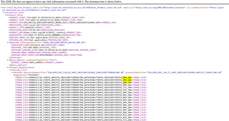
📜 Read the Metadata File and Extract URL Path
After downloading the metafile, we will read and extract the URL paths highlighted in the snapshot. For this article, the focus is on displaying the satellite image in RGB mode (Band 4, 3, and 2, respectively). However, if you wish to download other bands, such as SWIR bands, feel free to modify the following code and retrieve additional URL paths:
# Load XML2 library for XML processing
library(xml2)

# Read the MTD XML file
tree <- read_xml(outfile)
root <- xml_root(tree)

# Get paths for individual bands in Sentinel-2 granule
band_path <- list()
for (i in 1:4) {
  band_path[[i]] <- strsplit(paste0(product_name, "/", xml_text(xml_find_all(root, ".//IMAGE_FILE"))[i], ".jp2"), "/")[[1]]
}

# Display band paths
for (band_node in band_path) {
  cat(band_node[2], band_node[3], band_node[4], band_node[5], band_node[6], "\n")
}
The URL paths will be:

📥 Download the “jp2” files
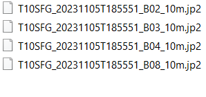
With the URLs path and the generated token, we can download each band separately into the desired directory. The following lines will download Bands 2, 3, 4, and 8, corresponding to Blue, Green, Red, and NIR, in “jp2” format:
# Build URLs for individual bands and download them
for (band_node in band_path) {
  url_full <- paste0(url_dataspace, "/Products(", product_id, ")/Nodes(", product_name, ")/Nodes(", band_node[2], ")/Nodes(", band_node[3], ")/Nodes(", band_node[4], ")/Nodes(", band_node[5], ")/Nodes(", band_node[6], ")/$value")
  print(url_full)

  # Perform GET request and handle redirects
  response <- GET(url_full, headers, config = httr::config(followlocation = FALSE))

  if (status_code(response) %in% c(301, 302, 303, 307)) {
    url_full_location <- response$headers$location
    print(url_full_location)
  }

  # Download the file
  file <- httr::GET(url_full_location, headers, config = httr::config(ssl_verifypeer = FALSE, followlocation = TRUE))
  print(status_code(file))

  # Save the product
  outfile <- file.path(getwd(), band_node[6])
  writeBin(content(file, "raw"), outfile)
  cat("Saved:", band_node[6], "\n")
}
These files will be downloaded and saved in your directory:
🛠️ Read the “jp2” files, Stack, and Clip to AOI
Before plotting the Sentinel-2 image, we clip the image for the Area of Interest (AOI). To do it, in the following lines, we will list the path of each band saved in our directory, read the projection of one of them, reproject our AOI to the same projection as the raster file, clip the raster file to our AOI, and stack the bands to create a single file with three bands (Blue, Green, and Red):
# Set the folder path
folder_path <- getwd()

# List all files with the ".jp2" extension
jp2_files <- list.files(path = folder_path, pattern = "\\.jp2$", ignore.case = TRUE, full.names = TRUE)

# Print the list of files
print(jp2_files)

# Extract Blue, Green, and Red bands based on their file names
blue_band  <- jp2_files[grep("_B02_", jp2_files)]
green_band <- jp2_files[grep("_B03_", jp2_files)]
red_band   <- jp2_files[grep("_B04_", jp2_files)]

# List the specific raster files
file_list <- c(blue_band, green_band, red_band)

# Define the AOI polygon
aoi_polygon <- "POLYGON ((-121.0616 37.6391, -120.966 37.6391, -120.966 37.6987, -121.0616 37.6987, -121.0616 37.6391))"

# Read and convert the AOI polygon to an sf object
aoi <- st_as_sfc(aoi_polygon)
#aoi <- st_read(aoi)

# Define the initial CRS for the AOI polygon (assuming it's in WGS84, EPSG:4326)
aoi <- st_set_crs(aoi, 4326)

# Read the first raster file to get its projection
raster_file <- raster(file.path(file_list[1]))
raster_projection <- projection(raster_file)

# Reproject the AOI polygon to match the raster projection
aoi_transformed <- st_transform(aoi, raster_projection)

# Read, clip, and stack the raster files
raster_list <- lapply(file_list, function(file) {
  raster_file <- raster(file)
  raster_clipped <- crop(raster_file, st_bbox(aoi_transformed))
  return(raster_clipped)
})

raster_stack <- stack(raster_list)
📈 Plot the True Color of the Surface Reflectance Image
Plotting can be done with one line of code:
# Plot the stacked raster
plot(raster_stack)
However, the output will be an individual plot for each band:
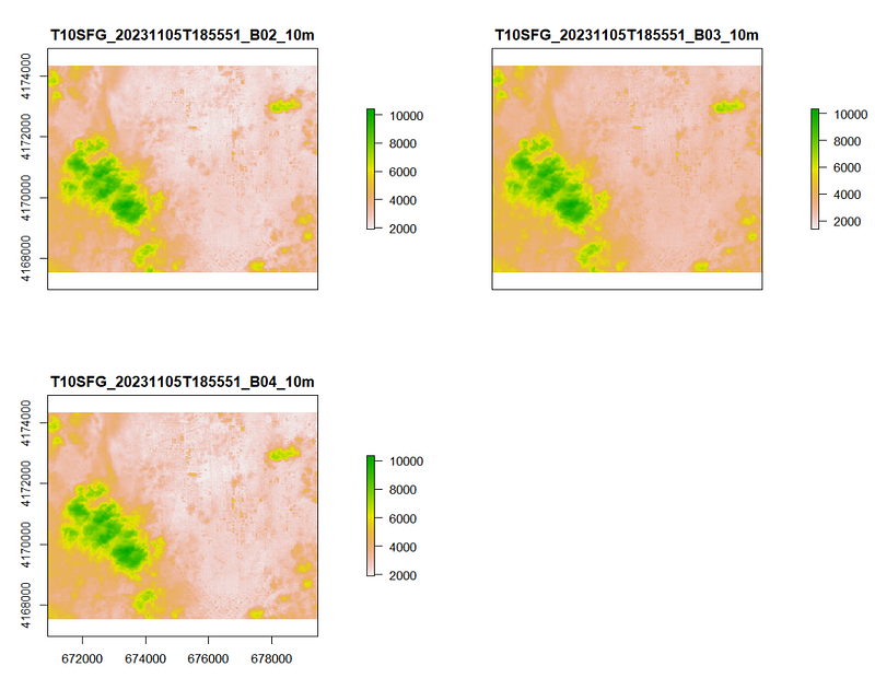
To fix this issue and display the image as a composite RGB image, we will read each band from the stacked file, normalize the bands by applying a gain factor, stack them again, and use the plotRGB function:
# Extract individual bands from the stacked raster
blue <- raster_stack[[1]]
green <- raster_stack[[2]]
red <- raster_stack[[3]]
# Set gain for better visualization
gain <- 3
# Normalize the bands and apply gain
blue_n <- clamp(blue * gain / 10000, 0, 1)
green_n <- clamp(green * gain / 10000, 0, 1)
red_n <- clamp(red * gain / 10000, 0, 1)
# Create an RGB composite
rgb_composite_n <- brick(red_n, green_n, blue_n)
# Plot the RGB composite
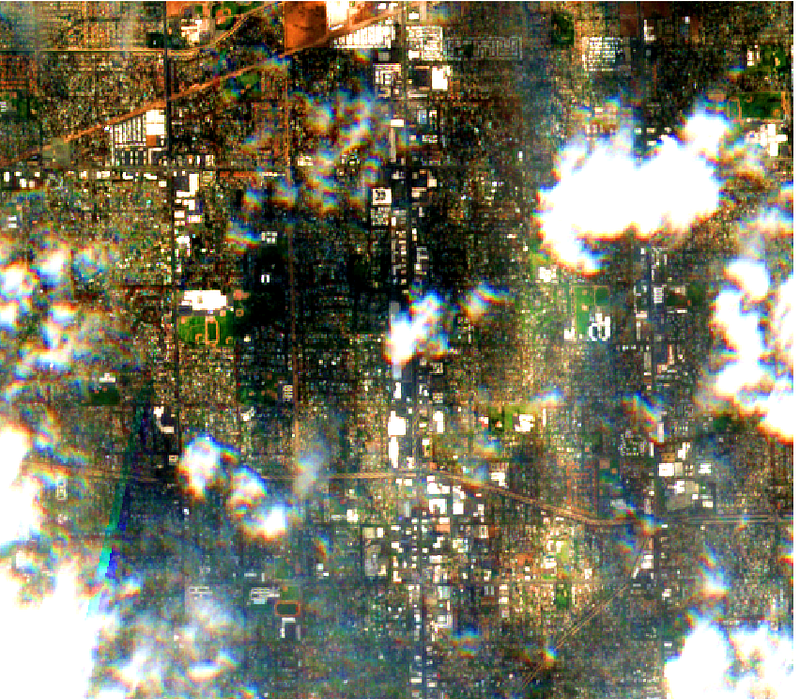
plotRGB(rgb_composite_n, scale = 1, stretch = "lin")The resulting map will be a nice snapshot captured by Sentinel-2 over an urban area, surrounded by many clouds on November 5th, 2023:
📚 References
https://documentation.dataspace.copernicus.eu/APIs/OData.html
- 👏 Be sure to clap for this article if you find it enjoyable.
- 📚 Hit that “Follow” button to stay updated on my latest posts.
- 🤝 Your feedback and engagement fuel my passion for sharing meaningful content.
- 📱 Also, connect with me on other platforms for more engaging content! LinkedIn, ResearchGate, Github, and Twitter.
You can explore my other stories through these links:


