START GUIDE

How to deal with an imbalanced dataset

Models trained on imbalanced datasets tend to perform poorly on minority classes because most machine learning algorithms for classification assume the classes are balanced. Not treating the imbalanced datasets correctly and not using correct metrics for model evaluation can cause severe problems if business decisions rely on the model’s outcome. This article shows few tricks when working with such datasets.

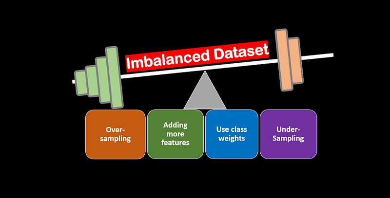
Classification algorithms are machine learning techniques that involve categorizing data into classes. It is one of the kinds of supervised machine learning, in which algorithms learn from labeled data. Since algorithms learn from the labeled data, hence the distribution of classes plays an important role. For example, training algorithms on the severely skewed dataset, also known as imbalanced datasets, can result in algorithms that perform poorly on minority classes. Fraud detection, churn prediction, spam detection are real-world examples of the imbalanced dataset. Therefore, building algorithms to tackle such imbalanced datasets requires special techniques to handle the distribution of the dataset and choosing the right evaluation metrics.

How to treat an imbalanced dataset?

In the real world, most of the datasets are not quite balanced. The figure below shows the three cases of imbalanced datasets.

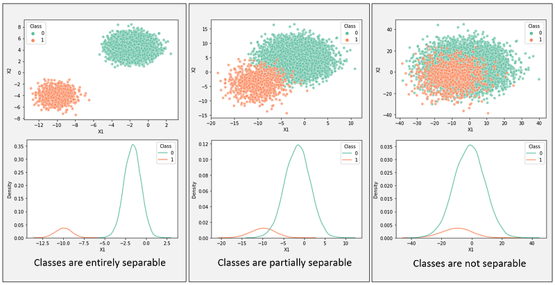
Figure showing examples of different scenarios of the imbalanced dataset.

In the figure above, Class 0 represents the majority class, and Class 1 represents the minority. If the classes are entirely separable, there is a high probability that this case can compensate for the imbalance. However, if the two classes overlap each other completely or partially, the majority class has a consistently higher probability than the minority class of being chosen.

Assuming the imbalance in the dataset represents reality, there are several ways to deal with imbalanced datasets before fitting the classifier in such cases.

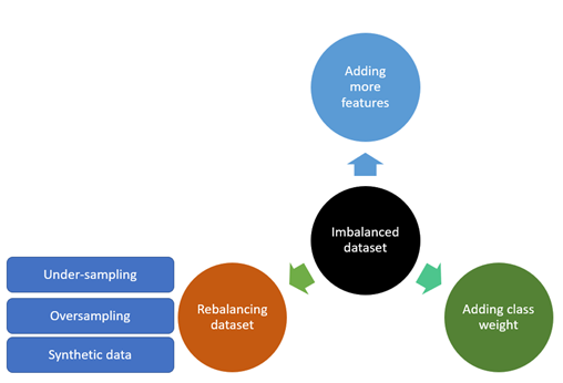
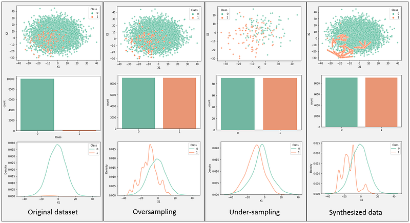
Figure showing ways of dealing with the imbalanced dataset.

The most widely used technique for imbalanced datasets is under-sampling, oversampling, or generating synthetic data. For example, the figure below shows different methods of making the imbalanced dataset balanced.

Figure showing ways of rebalancing dataset.

However, penalizing classifiers by applying more weights to the minority class or adding more input features that can separate the overlapping classes can be more effective in some cases rather than rebalancing the dataset.

Why is accuracy may not be a good choice for an imbalanced dataset?

Using accuracy as a metric for an imbalanced dataset is misleading. For example, a dataset for banking transactions has more than 99% data with non-fraudulent cases. Therefore, if a classifier only predicts transactions as non-fraudulent, still the classifier’s accuracy is 99%, which can be detrimental when such a model is deployed in the real world, leading to fraudulent transactions remaining undetected. Hence, to overcome the accuracy paradox, evaluation metrics such as precision, recall, f1-score, ROC, and AUC curves can provide more insight into model performance.

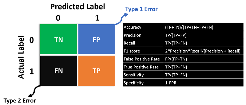
Figure showing different evaluation metrics.

Choosing the right metric also depends on the problem domain. For example, minimizing false negatives would lower the fraudulent case in credit card fraudulent problem; however, minimizing false-positive is also required; otherwise, many non-fraudulent cases would be detected fraudulent. Hence, in this case, the F1 score can be an excellent metric. The area under the curve (AUC) of receiver operating characteristics (ROC) is also an exciting metric that can show the model’s effectiveness. AUC closer to 1 means the model is highly effective.

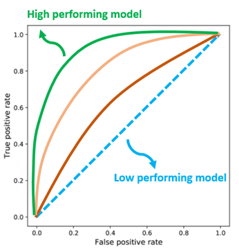
Figure showing the effectiveness of the model from low to high performing.

As shown in the figure above, a ROC curve close to the blue line suffers from low precision (high false positives) to get a high recall. On the other hand, as the ROC curve moves away from the blue line and closer towards the green line model becomes highly effective.

Working with Imbalanced dataset: Fraud detection classifier

About Dataset:

The credit card fraudulent dataset is a classic example of an imbalanced dataset that contains only 0.17% fraudulent cases (positive class). The dataset contains PCA transformed features (V1, V2, V3….V28) representing the original customer information. The amount input feature is not transformed and represents the transaction amount. The target label (Class) represents fraudulent (Class = 1) and Non-Fraudulent (Class = 0) case.

Exploratory Data Analysis:

The figure below shows the distribution of classes.

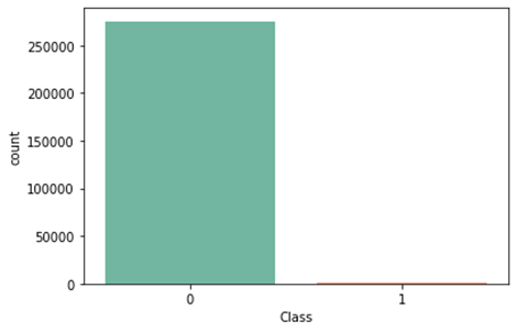
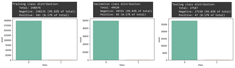
The dataset contains 275663 samples, out of which 275190 samples (99.83%) belong to non-fraudulent cases, and 473 samples (0.17%) belong to fraudulent cases. The figure below shows the correlation between the input features.

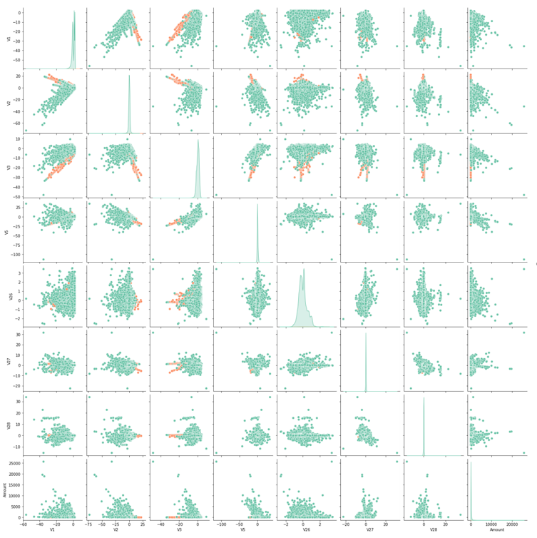
Figure showing the correlation between input features.

The figure above shows all input feature needs scaling. For example, the figure below is the distribution of the Amount input feature for both classes.

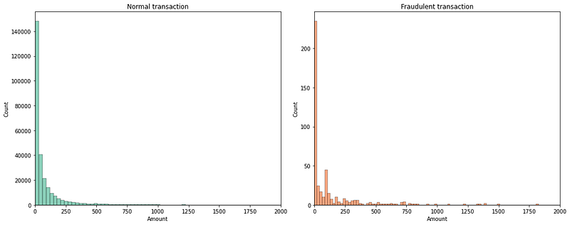
Figure showing the distribution of Amount input features.

The Amount input feature is heavily skewed. The figure below shows the Amount feature after log transformation.

Figure showing the distribution of Amount input features after log transformation.

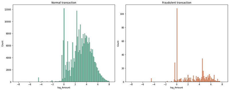
Before performing the standard scaling, split the dataset into three: train, validation, and test dataset. Use a stratification technique to preserve the distribution of classes in each group.

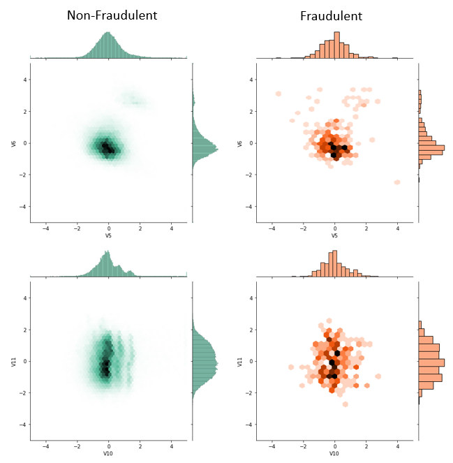
Figure showing the distribution of data between three groups.

Now, it is time for feature scaling and removal of outliers from the dataset. The figure below shows the few jointplots between input features for both classes.

Figure showing the distribution of data after rescaling.

The figure below shows that the distribution of the Amount feature after log transformation and feature scaling.

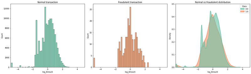
Figure showing the distribution of Amount feature after rescaling.

After fundamental exploratory data analysis and data cleaning, one can see that both classes are not separable. Hence it is a good idea to try different techniques such as applying class weights and rebalancing techniques to see which model performs best.

Model structure:

The model consists of four layers. A dropout layer reduces the overfitting, and the output layer uses sigmoid as an activation function to classify between negative and positive classes.

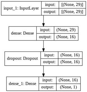
This article evaluates the performance of the model by feeding a balanced dataset using different rebalancing techniques. Also, methods like applying higher weight to the minority class have been explored and compared. However, in all the cases, the structure of models remains the same, as shown above.

Baseline model:

Since the dataset is imbalanced and classes are not separable, it is always good to start with a model without rebalancing and seeing how different metrics are performing in such a case. This model is a baseline and is used to measure the performance of other techniques. The figure below is the distribution of data based on both classes.

The figure below shows the baseline model performance.

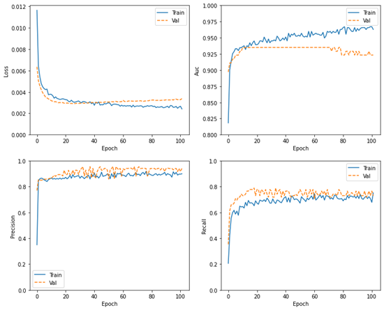
Figure showing evaluation metric for the baseline model.

The figure above shows that the precision of the baseline model is higher than the recall. Low recall means that model is struggling with classifying fraudulent cases. Also, after the 50 epochs loss curve, validation loss is increasing, which signals to overfit the data.

Class weights:

The first way to tackle imbalance in the dataset is by penalizing the model when it cannot predict the minority class (false negatives). Use the following for the calculation of weights.

In this case, the model trained without balancing the dataset.

Figure showing the distribution of data points on which weighted class model built.

The figure below shows the model performance with a weighted class.

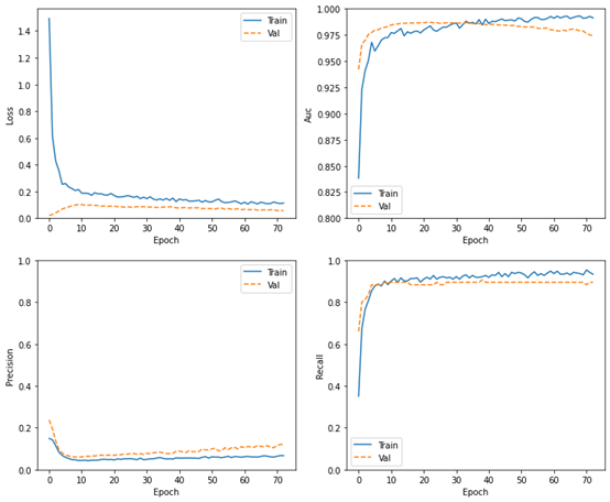
Figure showing evaluation metric for the model with weighted class.

The figure above shows that the precision of the weighted class model is lower than the recall. High recall means that this model was focusing more on predicting the fraudulent case.

Oversampling minority class using duplicates:

The other way to approach the problem is through oversampling. In this case, the minority class data points replicated to match the majority class sample size. The figure below shows the distribution of oversampled data.

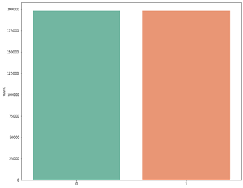
Figure showing the distribution of data points on which oversampled model built.

The figure below shows the model performance with an oversampling.

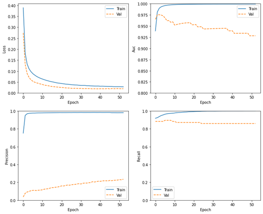
Figure showing evaluation metric for the model with oversampled class.

The figure above shows that the precision in the training dataset is higher compared to the validation dataset. Without any class weights, just rebalancing the dataset leads to high recall.

Oversampling minority class using SMOTE:

Generating synthetic data is another approach to oversample the minority class. The advantage of such techniques is that instead of learning from the duplicate sample, the model sees some variation in minority class, making it more generalizable. The figure below shows the distribution of oversampled data.

Figure showing the distribution of data points on which oversampled model built using SMOTE.

The figure below shows the model performance with an oversampling using SMOTE.

Figure showing evaluation metric for the model with oversampled class with SMOTE.

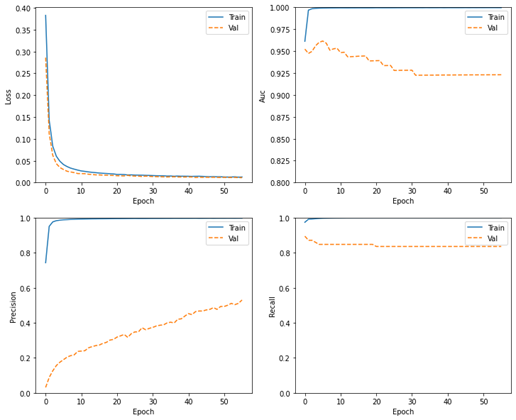
The figure above shows that the precision increases with the number of epochs and higher than the precision offered by oversampling using duplicates.

Under-sampling majority class:

Another approach is under-sampling the majority class to make the number of samples equal to the minority class. The figure below shows the distribution of under-sampled data.

Figure showing the distribution of data points on which under-sampled model built.

The figure below shows the model performance with an under-sampling method.

Figure showing evaluation metric for the model with the under-sampling method.

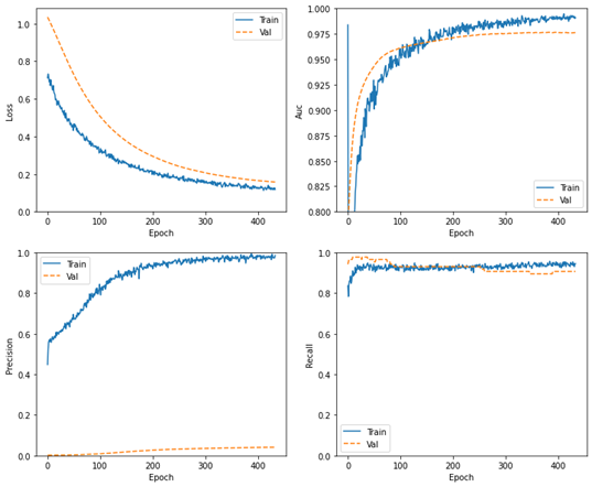
The figure above shows that the precision for validation data is low.

Model comparison:

ROC curve: The ROC curve shown below shows the comparison between different training and test dataset techniques.

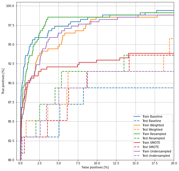
Figure showing ROC curve for different methods.

The figure above shows a large gap between training and test datasets regarding model performance for baseline, which hints at the overfitting issue. A model with a weighted class performs much better on test data; sacrificing little on precision leads to higher recall in this case. However, using synthetic data (SMOTE) and resampling (oversampling using duplicate) shows good performance.

Note: This is just an example; one should also try cross-validation to see the average score of the evaluation metric because here, the samples were drawn randomly for over and under-sampling, which may affect the result. Hence, it is a good idea to look for deviation in results.

Confusion matrix: The confusion matrix shown below shows the comparison between different techniques on the test dataset.

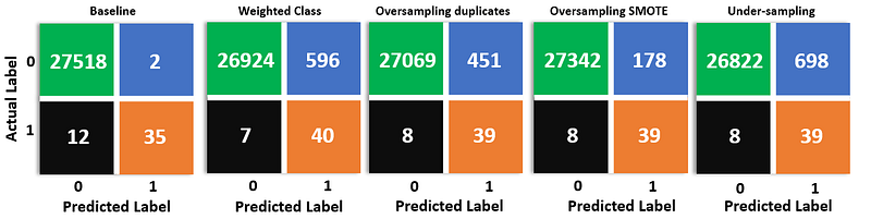
The above figure shows that the baseline model has a lower recall than the others, while precision is much higher because it has seen an imbalanced dataset. Thus, bias in data is reflecting in the result. Penalizing through class weights results in a higher recall, but precision suffers. Similarly, balancing the dataset results in a higher recall, but the model trained with synthetic data created using SMOTE shines. Instead of creating duplicates of the minority class, it introduces some noise, which helps the model generalize better.

Note: The accuracy of all the tests is between 97–99% which is misleading, as discussed before.

Summary

The following points were covered in this article when working with imbalanced datasets.

Most real-world problems might suffer from some imbalance in the dataset. In such cases, using accuracy as a metric might be misleading.
The imbalance in the dataset may vary from slight to severe; the more severe the imbalance, the more challenging the problem becomes.
Gathering more features for an imbalanced dataset may be helpful.
If the classes in the dataset are separable, it may compensate for the imbalance in the dataset.
If classes are not separable, then adding weights to penalize the model not predicting the minority class or class rebalancing using under-sampling oversampling should be explored.
Different models such as isolation forest could also be an alternate solution for such cases.
Oversampling with data augmentation may help for the model to generalize better.

I hope you enjoyed this article. Any questions? Have I missed something? Please reach out on my LinkedIn or Twitter.

Follow this Github link to access all the resources used for this article.

Cheers!

Rahul