How to Choose the Best Evaluation Metric for Classification Problems

A comprehensive guide covering the most commonly used evaluation metrics for supervised classification and their utility in different scenarios

In order to properly evaluate a classification model, it is important to carefully consider which evaluation metric is the most suitable.

This article will cover the most commonly used evaluation metrics for classification tasks, including relevant example cases, and will provide you with the information necessary to help you choose among them.

Classification

A classification problem is characterized by the prediction of the category or class of a given observation based on its corresponding features. The choice of the most appropriate evaluation metric will depend on the aspects of model performance the user would like to optimize.

Imagine a prediction model aiming to diagnose a particular disease. If this model fails to detect the disease, it can lead to serious consequences, such as delayed treatment and patient harm. On the other hand, if the model falsely diagnoses a healthy patient, that can also result in costly consequences by subjecting a healthy patient to unnecessary tests and treatments.

Ultimately, the decision on which error to minimize will depend on the particular use case and the costs associated with it. Let’s go through some of the most commonly used metrics to shed some more light on this.

Evaluation Metrics

Accuracy

When the classes in a dataset are balanced—meaning if there is roughly an equal number of samples in each class — accuracy can serve as a simple and intuitive metric to evaluate a model’s performance.

In simple terms, accuracy measures the proportion of correct predictions made by the model.

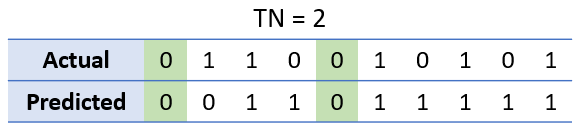
To illustrate this, let’s have a look at the following table, showing both actual and predicted classes:

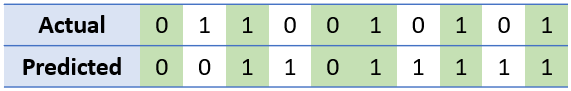
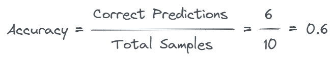
In this example, we have a total of 10 samples, of which 6 have been predicted correctly (green shading).

Thus, our accuracy can be calculated as follows:

In order to prepare ourselves for what’s about to come with the metrics below, it is worth noting that correct predictions are the sum of true positives and true negatives.

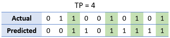
A true positive (TP) occurs when the model correctly predicts the positive class.

A true negative (TN) occurs when the model correctly predicts the negative class.

In our example, a true positive is an outcome where both actual and predicted classes are 1.

Likewise, a true negative occurs when both actual and predicted classes are 0.

Therefore, you may occasionally see the formula for accuracy being written as follows:

Example: Face detection. In order to detect the absence or presence of a face in an image, accuracy can be a suitable metric as the cost of a false positive (identifying a non-face as a face) or a false negative (failing to identify a face) is approximately equal. Note: the distribution of the class labels in the dataset should be balanced in order for accuracy to be an appropriate measure.

Precision

The precision metric is suitable for measuring the proportion of correct positive predictions.

In other words, precision provides a measure of the model’s ability to correctly identify true positive samples.

As a result, it is often used when the goal is to minimize false positives, as is the case in domains like credit card fraud detection or disease diagnosis.

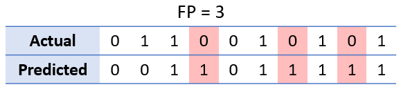
A false positive (FP) occurs when the model incorrectly predicts the positive class, indicating that a given condition exists when in reality it does not.

In our example, a false positive is an outcome where the predicted class should have been 0, but was actually 1.

Since precision measures the proportion of positive predictions that are actually true positives, it is calculated as follows:

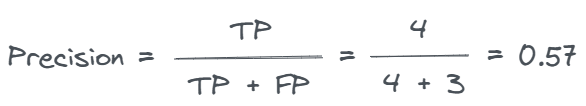
Example: Anomaly detection. In fraud detection, for instance, precision can be a suitable evaluation metric, particularly when the cost of false positives is high. Identifying non-fraudulent activities as fraudulent can lead not only to additional costs for investigation expenses, but also to high levels of customer dissatisfaction and increased churn rates.

Recall

When the goal of a prediction task is to minimize false negatives, recall serves as an appropriate evaluation metric.

Recall measures the proportion of true positives that are correctly identified by the model.

It is particularly useful in situations where false negatives are more costly than false positives.

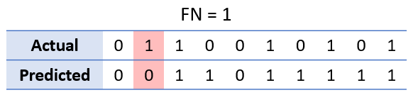
A false negative (FN) occurs when the model incorrectly predicts the negative class, indicating that a given condition is absent when in fact it is present.

In our example, a false negative is an outcome where the predicted class should have been 1, but was actually 0.

Recall is calculated as follows:

Example: Disease diagnosis. In COVID-19 testing, for instance, recall is a good choice when the goal is to detect as many positive cases as possible. In this case, a higher number of false positives is tolerated since the priority is to minimize false negatives in order to prevent the spread of the disease. Arguably, the cost of missing a positive case is much higher than misclassifying a negative case as positive.

F1 Score

In cases when both false positives and false negatives are important aspects to consider, such as in spam detection, the F1 score comes in as a handy metric.

The F1 score is the harmonic mean of precision and recall and provides a balanced measure of the model’s performance by taking into account both false positives and false negatives.

It is calculated as follows:

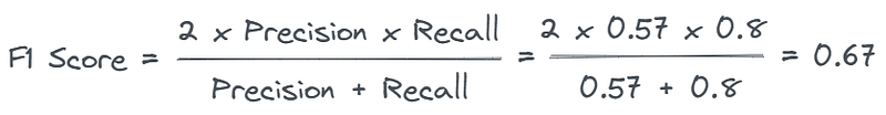
Example: Document classification. In spam detection, for instance, the F1 score is an appropriate evaluation metric, as the goal is to strike a balance between precision and recall. A spam email classifier should correctly classify as many spam emails as possible (recall), whilst also avoid the incorrect classification of legitimate emails as spam (precision).

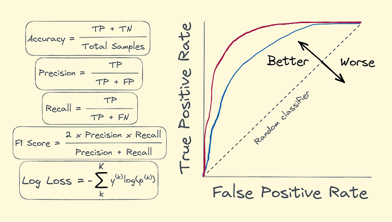
Area under the ROC curve (AUC)

The receiver operating characteristic curve, or ROC curve, is a graph that illustrates the performance of a binary classifier at all classification thresholds.

The area under the ROC curve, or AUC, measures how well a binary classifier can tell apart positive and negative classes across different thresholds.

It is a particularly useful metric when the cost of false positives and false negatives is different. This is because it considers the trade-off between true positive rate (sensitivity) and false positive rate (1-specificity) at different thresholds. By adjusting the threshold, we can get a classifier that prioritizes either sensitivity or specificity, depending on the cost of false positives and false negatives of a specific problem.

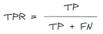
The true positive rate (TPR), or sensitivity, measures the proportion of actual positive cases that are correctly identified by the model. It is exactly the same as recall.

It is calculated as follows:

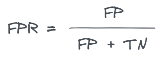
The false positive rate (FPR), or 1-specificity, measures the proportion of actual negative cases that are incorrectly classified as positive by the model.

It is calculated as follows:

By varying the classification threshold from 0 to 1, and calculating TPR and FPR for each of these thresholds, a ROC curve and corresponding AUC value can be produced. The diagonal line represents the performance of a random classifier — that is, a classifier that makes random guesses about the class label of each sample.

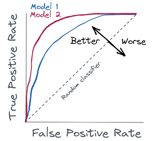
The closer the ROC curve is to the top left corner, the better the performance of the classifier. A corresponding AUC of 1 indicates perfect classification, whereas an AUC of 0.5 indicates random classification performance.

Example: Ranking problems. When the task is to rank samples by their likelihood of being in one class or another, AUC is a suitable metric as it reflects the model’s ability to correctly rank samples rather than just classify them. For instance, it can be used in online advertising, as it would evaluate the model’s ability to correctly rank users by their likelihood of clicking on an ad, rather than just predicting a binary click/no-click outcome.

Log Loss

Logarithmic loss, also known as log loss or cross-entropy loss, is a useful evaluation metric for classification problems where probabilistic estimates are important.

The log loss measures the difference between the predicted probabilities of the classes and the actual class labels.

It is a particularly useful metric when the goal is to penalize the model for being overly confident about predicting the wrong class. The metric is also used as a loss function in the training of logistic regressors and neural networks.

For a single sample, whereby y denotes the true label and p denotes the probability estimate, the log loss is calculated as follows:

When the true label is 1, the log loss as a function of predicted probabilities looks like this:

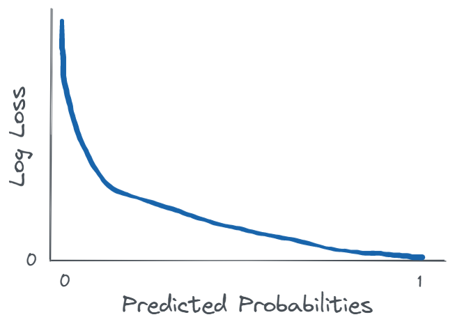
It can be clearly seen that the log loss gets smaller the more certain the classifier is about the correct label being 1.

The log loss can also be generalized to multi-class classification problems. For a single sample, where k denotes the class label and K corresponds to the total number of classes, it can be calculated as follows:

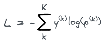
In both binary and multi-class classification, the log loss is a helpful measure that determines how well the predicted probabilities match the true class labels.

Example: Credit risk assessment. For instance, the log loss can be used to evaluate the performance of a credit risk model that predicts how likely a borrower is to default on a loan. The cost of a false negative (predicting a reliable borrower as unreliable) could be much higher than that of a false positive (predicting an unreliable borrower as reliable). Thus, minimizing the log loss can help minimize the financial risk of lending in this scenario.

Conclusion

In order to accurately assess the performance of a classifier and to make informed decisions based on its predictions, it is crucial to choose an appropriate evaluation metric. In most situations, this choice will highly depend on the specific problem at hand. Important factors to consider are the balance of the classes in a dataset, whether it’s more important to minimize false positives, false negatives, or both, and the significance of ranking and probabilistic estimates.

Liked this article?

Let’s connect! You can find me on Twitter, LinkedIn and Substack. If you like to support my writing, you can do so through a Medium Membership, which provides you access to all my stories as well as those of thousands of other writers on Medium.