How to change semi-structured text into a Pandas dataframe

Using Python and Pandas, I converted a text document meant for human readers into a machine readable dataframe

These days much of the data you find on the internet are nicely formatted as JSON, Excel files or CSV. But some aren’t.

I needed a simple dataset to illustrate my articles on data visualisation in Python and Julia and decided upon weather data (for London, UK) that was publicly available from the UK Met Office.

The problem was that it was a text file that looked like a CSV file but it was actually really formatted for a human reader. So, I needed to do a bit of cleaning and tidying in order to be able to create a Pandas dataframe and plot graphs.

This article is about the different techniques that I used to transform this semi-structured text file into a Pandas dataframe with which I could perform data analysis and plot graphs.

I could, no doubt, have converted the file with a text editor — that would have been very tedious. But I decided it would be more fun to do it programmatically with Python and Pandas. Also, and perhaps more importantly, writing a program to download and format the data meant that I could automatically keep it up to date with no extra effort.

There were a number of problems. First, there was the structure of the file. The data were tabulated but preceded by a free format description, so this was the first thing that had to go. Secondly, the column names were in two rows rather than the one that is conventional in a spreadsheet file. Then, although it looked a bit like a CSV file, there were no delimiters: the data were separated by a variable number of blank spaces.

Lastly, the number of data columns changed part way through the file. The data ranges from 1948 to the current time but the figures for 2020 were labelled ‘Provisional’ in an additional column.

Then there was the form of the data. In the early years some data were missing and that missing data was represented by a string of dashes. Other columns had a ‘#’ attached to what was otherwise numeric data. Neither of these could be recognised as numerical data by Pandas.

Each of these problems had to be addressed for Pandas to make sense of the data.

Reading the data

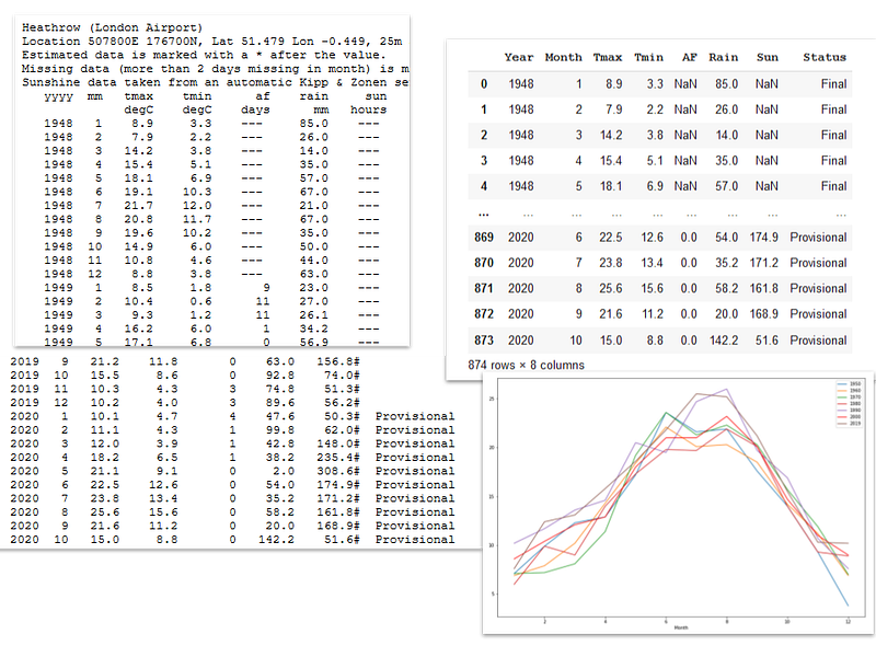
The data is in the public domain and provided by the Met Office as a simple text file. You can see the format in the image at the top of this article (along with the resulting dataframe and a graph drawn from the data).

Reading a csv file in Pandas is quite straightforward and, although this is not a conventional csv file, I was going to use that functionality as a starting point.

The function read_csv from Pandas is generally the thing to use to read either a local file or a remote one. Unfortunately, this did not work with the Met Office file because the web site refuses the connection. I’m not 100% sure but I imagine it is because it doesn’t like the ‘User Agent’ in the HTTP header supplied by the function (the user agent is normally the name/description of the browser that is accessing the web page — I don’t know, offhand, what read_csv sets it to).

I’m not aware of any mechanism that will allow me to change the User Agent for read_csv but there is a fairly simple way around this: use the requests library. (The requests library lets you set the HTTP headers including the User Agent.)

Using requests you can download the file to a Python file object and then use read_csv to import it to a dataframe. Here’s the code.

First import the libraries that we will use:

import pandas as pd
import matplotlib.pyplot as plt
import requests
import io

(If you have any missing you’ll have to conda/pip install them.)

And here is the code to download the data:

url = 'https://www.metoffice.gov.uk/pub/data/weather/uk/climate/stationdata/heathrowdata.txt'

file = io.StringIO(requests.get(url).text)

Just a minute, didn’t I say that I was going to set the User Agent? Well, as it happens, the default setting that requests uses appears to be acceptable to the Met Office web site, so without any further investigation, I just used the simple function call you see above. The requests call gets the file and returns the text. That is then converted to a file object by StringIO.

Fixing the structure

Now we are nearly ready to read the file. I needed to take a look at the raw file first and this showed me that the first 5 lines were unstructured text. I would need to skip those lines to read the file as csv.

The next two lines were the column names. I decided to skip those, too, and provide my own names. Those names are ‘Year’, ‘Month’, ‘Tmax’, ‘Tmin’, ‘AF’, ‘Rain’, ‘Sun’. The first two are obvious, Tmax and Tmin are the maximum and minimum temperatures in a month, AF is the number of days when there was air frost in a month, Rain is the number of millimeters of rain and Sun is the number of hours of sunshine.

I recorded these things in variables like this:

col_names = ('Year','Month','Tmax','Tmin','AF','Rain','Sun')
comment_lines = 5
header = 2

These will be used in the read_csv call.

read_csv needs some other parameters set for this particular job. It needs to know the delimiter used in the file, the default is a comma (what else?) but here the delimiter is a space character, in fact more than one space character. So, I need to tell pandas this (delimiter=` ´). And because there are several spaces between the fields, Pandas needs to know to ignore these (skipinitialspace=True).

I need to tell it that it should skip the first few rows (skiprows=comment_lines+header), not regard any row in the file as a header (header=None) and the names of the columns (names=col_names).

Finally, I know that when it gets to the year 2020 the number of columns change. This would normally throw an exception and no dataframe would be returned. But setting error_bad_lines=False suppresses the error and ignores the bad lines.

Here is the resulting code that creates the dataframe weather.

weather = pd.read_csv(file,
   skiprows=comment_lines + header,
   header=None,
   names=col_names,
   delimiter=' ',
   skipinitialspace=True,
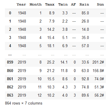
   error_bad_lines=False)

That produces a dataframe that contains all the data up the first bad line (the one with the extra column).

The individual data items need fixing but the next job is to append the rest of the file. This time I’ll read the file again, using similar parameters but I’ll find the length of the dataframe that I’ve just read and skip all of those lines. The remaining part of the file contains 8 columns, so I need to add a new column name as well. Otherwise the call to read_csv is similar to before.

file.seek(0)

col_names = ('Year','Month','Tmax','Tmin','AF','Rain','Sun', 'Status')
rows_to_skip = comment_lines+header+len(weather)

weather2 = pd.read_csv(file,
   skiprows=rows_to_skip,
   header=None,
   names=col_names,
   delimiter=' ',
   skipinitialspace=True,
   error_bad_lines=False)

Also, notice that I had to set the pointer back to the beginning of the file using seek(0) otherwise there would be nothing to read as we already had reached the end of the file.

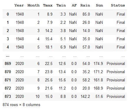
Here’s the result:

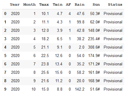
Similar to the other dataframe but with an extra column.

The next trick is to merge the two dataframes and to do this properly I have to make them the same shape. So, I have a choice, delete the Status column in the second dataframe or add one to the first dataframe. For the purposes of this exercise, I’ve decided to not lose the status information and add a column to the first. The extra column is called Status and for the 2020 data its value is ‘Provisional’. So, I’ll create a Status column in the first dataframe and set all the values to ‘Final’.

weather['Status']='Final'

And now I’ll append the second dataframe to the first and add the parameter ignore_index=True in order not to duplicate the indices but rather create a new index for the combined dataframe.

weather = weather.append(weather2, ignore_index=True)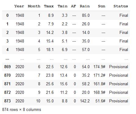

Fixing the data types

Now we have to deal with the data in each column. Let’s take a look at the data types.

weather.dtypes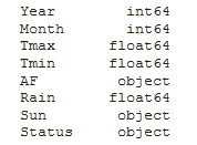

As you can see, Pandas has done its best to interpret the data types: Tmax, Tmin and Rain are correctly identified as floats and Status is an object (basically a string). But AF and Sun have been interpreted as strings, too, although in reality they ought to be numbers. The reason for this is that some of the values in the Sun and AF columns are the string ‘ — -’ (meaning no data) or the number has a # symbol attached to it.

It’s only the Sun column that has the # symbol attached to the number of hours of sunshine, so the first thing is to just get rid of that character in that column. A string-replace does the job; the code below removes the character by replacing it with an empty string.

weather['Sun']=weather['Sun'].str.replace('#','')

Now the numbers in the Sun column are correctly formatted but Pandas still regards the Sun and AF columns data as strings so we can’t read the column as numbers and cannot therefore draw charts using this data.

Changing the representation of the data is straightforward; we use the function to_numeric to convert the string values to numbers. Using this function the string would convert the string “123.4” to a floating point number 123.4. But some of the values in the columns that we want to convert are the string ‘ — -’, which cannot be reasonably interpreted as a number.

The trick is to set the parameter errors to coerce. This will force any strings that cannot be interpreted as numbers to the value NaN (not a number) which is the Python equivalent of a null numeric value. And this is exactly what we want because the string ‘ — -’ in this dataframe means ‘no data’.

Here is the code to correct the values in the two columns.

weather['AF']=pd.to_numeric(weather['AF'], errors='coerce')
weather['Sun']=pd.to_numeric(weather['Sun'], errors='coerce')

The dataframe now looks like this:

You can see the NaN values and if we look at the data types again we see this:

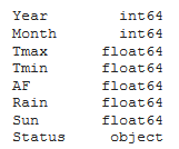
Now all of the numeric data are floating point values — exactly what is needed.

Using the data

To illustrate that this is what we want here is a plot of the rainfall for the year 2000.

weather[weather.Year==2000].plot(x='Month', y='Rain')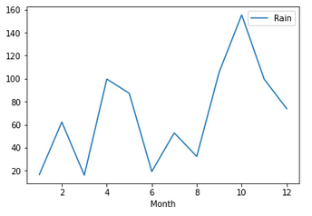

Job done!

And if you are wondering where the graph at the top of this article comes from, here is the code that plots the monthly maximum temperatures for 1950, 1960, 1970, 1980,1990, 2000 and 2010.

ax = weather[weather.Year==1950].plot(x='Month', y='Tmax',
   label='1950')
ax = weather[weather.Year==1960].plot(x='Month', y='Tmax', 
   label='1960',ax=ax)
ax = weather[weather.Year==1970].plot(x='Month', y='Tmax',  
   label='1970',ax=ax)
ax = weather[weather.Year==1980].plot(x='Month', y='Tmax', 
   label='1980',ax=ax)
ax = weather[weather.Year==1990].plot(x='Month', y='Tmax', 
   label='1990',ax=ax)
ax = weather[weather.Year==2000].plot(x='Month', y='Tmax', 
   label='2000',ax=ax)
weather[weather.Year==2019].plot(x='Month', y='Tmax', label = 
   '2010', ax=ax, figsize=(15,10));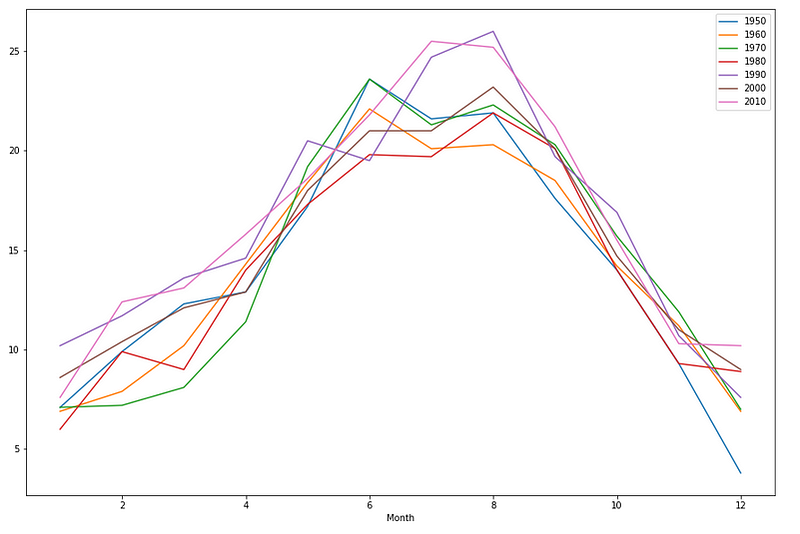

It is unlikely that you will find that you need to do exactly the same manipulations on a text file that I have demonstrated here but I hope that you may have found my experience useful and that you may be able to adapt the techniques that I have used here for your own purposes.

Thanks for reading and if you would like to keep up to date with the articles that I publish, please consider subscribing to my free newsletter here.

Update: I have written a new more generic version of the above program here.