How to Build Quant Algorithmic Trading Model in Python

A step-by-step guide to perform Alpha Research in python

This post covers the basics of the alpha research process. ziplineand alphalens are used to manage the pipeline and measure the performance in a way to be explicit about the quantitative process. You can check zipline tutorial as well.

The focus of this post is on pure alpha research process and I will cover the backtesting (How to Perform Backtesting in Python — added on 14 Jan 2021) and utilisation of AI/machine learning in another post later (How to generate AI Alpha Factor in Python — added on 26 Dec 2020). Also, as a matter of course, the model described in this post is just a sample and should not be used in production.

1. Data Preparation

Ingesting Data

The first step is to get necessary data. zipline provides ingestion function to get data from their bundle or create a custom data bundle. Once zipline is installed, you can simply execute this to get a default data bundle sourced from Quandl and preprocessed by Quantopian.

Then the ingested data can be loaded by bundles.load() function. Instead of the default bundle, I use a specific data set here to match with a pre-defined sector classification.

Selecting Universe and Returns

Depending on the strategy, select which assets to consider in the portfolio. As the transaction cost is higher and not always possible to execute the strategy for illiquid assets, select top 500 US Stocks in terms of ADV. Note that when doing the full-backtesting, the universe should be constructed based on the data available on each historical day, rather than just the end state as done here in order to avoid the survivorship bias.

Use daily closing price and define the return as the percent change in price from the previous day.

2. Risk Model

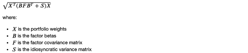
There are different ways to define the risk model but roughly speaking, it is to define the risk factors and measure the portfolio risk as the sum of exposure to those risk factors and unique risks that are not explained by the factors, which can be calculated asthe square root of the portfolio variance:

Statistical Risk Model

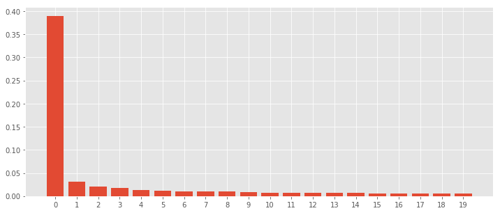
You can of course use one of the well-known factor models such as classic Fama-French Three-Factor Model or Five-Factor Model. Here, use Principal Component Analysis (PCA) to define the factors. In this example, the first component explains fairly large part of price variance.

Factor Betas

Factor Beta is the exposure of each asset in the universe to each component in PCA. Note that this is not exposures of your portfolio but the universe:

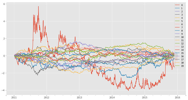
Factor Returns

Return of each risk factor (ie. components of PCA in this case) can be calculated as follows:

Factor Covariance Matrix

Covariance is a diagonal matrix, annualised by factor of 252 (=the number of trading days per year):

Idiosyncratic Variance Matrix and Vector

Residuals that are not explained by the 20 factors are considered as idiosyncratic to each asset.

Portfolio Risk

Assuming the portfolio evenly distribute the holdings to all the stocks in the universe, the portfolio risk can be calculated like this:

3. Alpha Factor

Let’s define three popular factors as alpha factors. In fact, alpha factors will become risk factors once they become publicly known and available and these are just for demonstration purpose. Also, it is important to be aware of the alpha factors should be the ones available during the data period to avoid look ahead bias, including the techniques and machine powers to generate the alpha signal.

Momentum 1 Year Factor

Momentum strategies are one of the most fundamental approaches that assumes the price trend will continue in the same direction. There are many ways to model this, such as trading at crossing points between different period of moving average. Here, simply take one-year return of each stock, demean the return by sector to be sector neutral, rank them and take z-score to avoid trading too much by normalisation. This is important to have a realistic signal that is stable enough to be profitable, which should be considered even before the full-backtesting.

Mean Reversion 5 Day Sector Neutral Smoothed Factor

Mean reversion is another popular strategy that assume big moves will partly reverse to the mean. It is a well known phenomenon in the financial market especially for stocks. This factor here takes the reverse order of 5-days return as signal and apply moving average of a month.

Overnight Sentiment Smoothed Factor

There are many papers published on the market phenomenon and keeping up with the recent development is also an important part of the process. As an example, here implements a factor introduced by this paper: Overnight Returns and Firm-Specific Investor Sentiment.

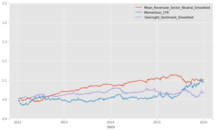
Performance: Factor Returns

First performance measurement is the factor return. alphalens provides useful functions to calculate the alpha performance.

Performance: Sharpe Ratio / Information Ratio (IC)

It cannot be judged whether the factor just from return. The return should be sufficient considering the risks taken; in other words, sharpe ratio should be around 1.5 to 2.0. Less than 1.0 is not good but also better to investigate if sharpe ratio is too good. IC = Sharpe Ratio for the market and common factor neutral portfolio, and our objective is to maximise Information Ratio (IR) = IC x sqrt(B) where B is breadth, the number of independent bets, so seeking for a good Sharpe Ratio is crucial.

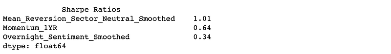
As expected, these factors themselves does not have good sharpe ratios.

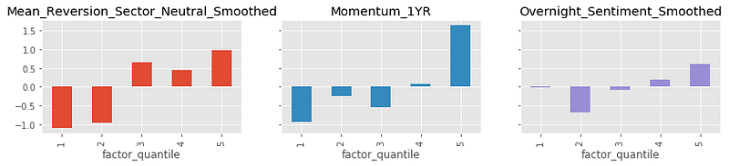
Performance: Quantile Analysis

Quantile Returns provide a good view on the portfolio whether all the assets in the portfolio are contributing to the returns. The graph should ideally be evenly rising to the right with point symmetry at 0 in the middle — monotonic in quantiles indicates Rank IC (i.e. Sharpe Ratio on ranked alpha values for market and common factor neutral portfolio) is highly correlated with forward future return.

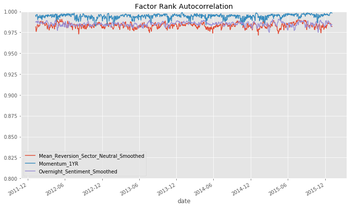
Performance: Turnover Analysis

The more stable the factor exposure, the better from transaction cost perspective. It can be checked by checking the factor rank autocorrelation (FRA), which indicates the factor with FRA close to 1 is correlate to the self well and does not require to trade a lot.

Combined Alpha Vector

Finally, a number of alpha factors should be combined to a single vector to decide which assets / how many stocks to buy or sell on each trading day. The weighted average based on sharpe ratio, or machine learning would be useful. Here just take the mean of all the alpha factors on the last day to demonstrate the portfolio optimisation described in the next section.

4. Portfolio Optimisation

Once we are confident that the combined alpha vector is promising, find a portfolio that trades as close as possible to the alpha model but limiting risk as measured by the risk model. Use CVXPY to solve optimisation problems.

Portfolio Constraints

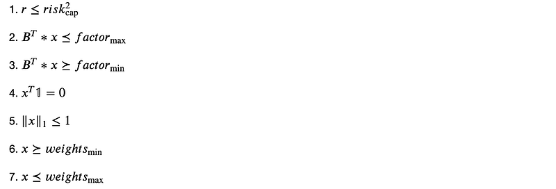
Given x is the portfolio weights, B is the factor betas and r is the portfolio risk, some of the typical constraints are:

1. The predicted risk must be less than some maximum limit
2. The maximum portfolio factor exposure
3. The minimum portfolio factor exposure
4. The market neutral constraint: the sum of the weights must be zero
5. The leverage constraint: the sum of the abolute value of the weights must be less than or equal to 1.0
6. The minimum limit on individual holdings
7. The maximum limit on individual holdings

Objective Function

Basically, the objective is to maximise alpha vector x portfolio weight:

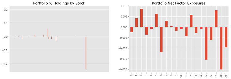
With this objective function, the portfolio is constructed with only a few stocks. There are ways to penalise this kind of allocation.

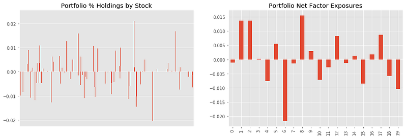
Optimize with Regularisation

In order to enforce diversification, use regularisation term in the objective function here. Given lambda as the regularisation parameter, the new objective function is to maximise this:

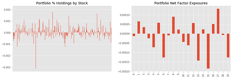
Optimize for Target Weight

Another approach to enforce the diversification is to minimise the deviation of portfolio weights x from the target weighting x*

Transfer Coefficient

Due to the optimisation with certain constraints, the actual trading and portfolio is no longer the one calculated from alpha signals. Therefore, it is also important to check how much the original idea is retained in the final trading by checking the correlation coefficient between alpha vector and the final portfolio weight.

Conclusion

We’ve gone through the basic alpha research process so far. This is just a very simple by leaving complex parts aside but effective way to quickly validate the alpha idea before the full-backtesting.

In the full-backtesting, the look-ahead bias, the transaction cost, etc. should be taken into consideration. In addition, commercial factor models and data from various providers including alternative data, which are sometimes unstructured, are inevitable to stay competitive, where the data wrangling also plays an important role (How to Perform Backtesting in Python — added on 14 Jan 2021).

Also, the application of machine learning techniques have become more common and usable. I will cover these parts later (How to generate AI Alpha Factor in Python — added on 26 Dec 2020).

It’s a pity that Quantopian ceased its operation in October 2020 and they shutdown the service. Another post will cover how to migrate to an alternative service and libraries such as QuantConnect/Lean.

The source code used in this post is available in github.