How to Build an AI-Powered Game Bot with PyTorch and EfficientNet

This article will guide you through creating an AI model that can play the popular Chrome Dino Game using PyTorch and EfficientNet.

OpenAI, the organization that developed ChatGPT, actually started by building AI models that could play Atari games. This project, known as the Atari AI, was one of the first demonstrations of deep reinforcement learning and helped pave the way for many subsequent advances in AI. So, building an AI model to play the Chrome Dino Game is part of a long tradition of using games to test and develop AI algorithms.

The Chrome Dino Game is a simple yet addictive game that has captured the hearts of millions of players worldwide. The game's objective is to control a dinosaur and help it run as far as possible without hitting obstacles. With the help of AI, we can create a model that can learn how to play the game and beat our high scores.

This tutorial is for anyone interested in building an AI model that can play games. Even if you are new to AI or deep learning, this tutorial will be a great starting point.

Using PyTorch, a popular deep learning framework, and EfficientNet, a state-of-the-art neural network architecture, we will train a model to analyze the game screen and make decisions based on what it sees. We will start by getting the necessary data, then processit, and finally train the model. By the end of this tutorial, you will have a better understanding of deep learning and how to train your own AI model.

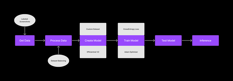
There are six major steps to setting up an AI model:

1. Getting the Data
2. Processing the Data
3. Creating the Model
4. Training the Model
5. Testing the Model
6. Inferring from the Model

• Install Anaconda: Download and install the Anaconda distribution from the official website for your operating system from here.
• Create a new project folder. Let’s name it “dino.” Open VS Code in this folder and open the terminal.
• Create a new conda environment: Open Anaconda Prompt or your terminal and create a new conda environment by running the following command:

conda create --name myenv python=3.10

This will create a new environment named myenv with Python 3.10 installed.

• Activate the environment: Once the environment is created, activate it using the following command:

conda activate myenv

• Install PyTorch: Install the PyTorch library with CUDA support (for GPU acceleration) using the following command:

conda install pytorch torchvision torchaudio cudatoolkit=11.1 -c pytorch -c conda-forge

• This command installs PyTorch, TorchVision, and TorchAudio with the CUDA toolkit version 11.1. You can change the version of the CUDA toolkit as per your requirement.
• Test the installation: To verify the PyTorch installation, run the following command to start a Python interpreter in your conda environment:

python

• Then, import the PyTorch library and print its version as follows:

import torch
print(torch.__version__)

This should print the version number of PyTorch installed in your environment.

Step 1: Getting the Data

We will get our data by taking snapshots of the game screen while a human player is playing the game. captures.py handles this.

import cv2
from PIL import ImageGrab
import numpy as np
import keyboard
import os
from datetime import datetime

current_key = ""
buffer = []

# check if folder named 'captures' exists. If not, create it.
if not os.path.exists("captures"):
    os.mkdir("captures")

def keyboardCallBack(key: keyboard.KeyboardEvent):
    '''
    This function is called when a keyboard event occurs. It stores the key pressed in a buffer and sorts it.

    ### Arguments : 
    `key (KeyboardEvent)`

    ### Returns : 
    `None`

    ### Example : 
    `keyboardCallBack(key)`
    '''

    global current_key

    if key.event_type == "down" and key.name not in buffer:
        buffer.append(key.name)

    if key.event_type == "up":
        buffer.remove(key.name)

    buffer.sort()  # Arrange the keys pressed in an ascending order
    current_key = " ".join(buffer)

keyboard.hook(callback=keyboardCallBack)
i = 0

while (not keyboard.is_pressed("esc")):

    # Capture image and save to the 'captures' folder with time and date along with the key being pressed
    image = cv2.cvtColor(np.array(ImageGrab.grab(
        bbox=(620, 220, 1280, 360))), cv2.COLOR_RGB2BGR)

    # if key pressed embed the key pressed in the file name
    if len(buffer) != 0:
        cv2.imwrite("captures/" + str(datetime.now()).replace("-", "_").replace(":",
                    "_").replace(" ", "_")+" " + current_key + ".png", image)

    # if no key pressed embed 'n' in the file name
    else:
        cv2.imwrite("captures/" + str(datetime.now()).replace("-",
                    "_").replace(":", "_").replace(" ", "_") + " n" + ".png", image)
    i = i+1

This code captures screenshots and saves them as PNG files in a specified directory. The screenshots are taken using the Python libraries PIL (Python Imaging Library) and OpenCV, and are captured using the ImageGrab module. The coordinates of the region to capture the screenshots are specified using the bbox (bounding box) argument in ImageGrab.grab. You might want to fiddle around with the bbox values based on your display scaling.

The program also captures keyboard events using the keyboard library. When a key is pressed, the name of the key is appended to a buffer. When the key is released, the name of the key is removed from the buffer. The current state of the buffer is saved as a string in the variable current_key.

The program saves each screenshot with a filename that contains the current value of i (an integer that is incremented with each iteration of the while loop) and the current state of the buffer (as saved in current_key). If no keys are pressed when the screenshot is taken, the filename includes “n” instead of a key name.

This code could be used as a starting point for building an image dataset for machine learning projects, such as object recognition or image classification. By capturing images and labeling them with the corresponding keys pressed, a dataset could be created that could be used to train a machine learning model to recognize the images and predict the corresponding key presses.

Head over to https://chromedino.com/ and start playing the game while the script captures the images and saves them to the “captures” folder.

Run this Python file and start playing the game. Play for at least 20 different runs to get a good dataset.

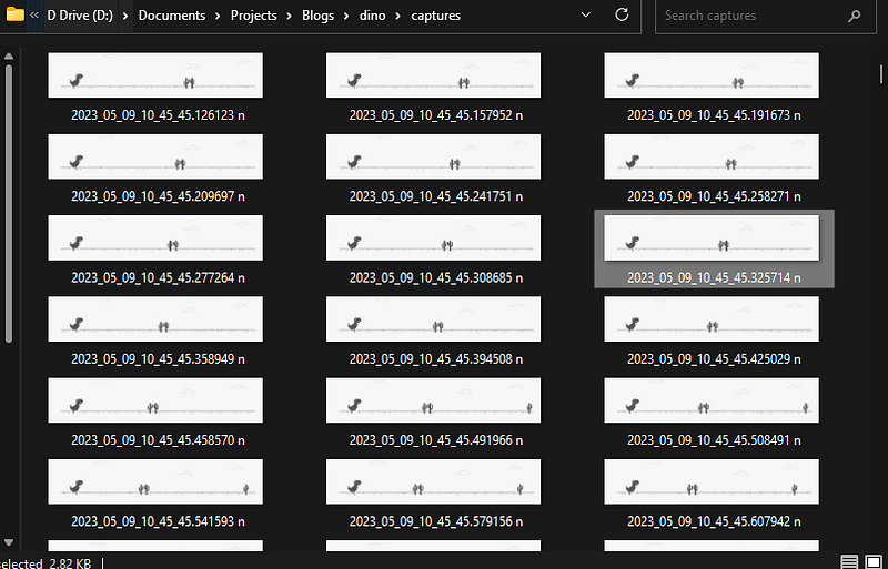
The captured image should look something like this:

This is how the “captures” folder should look once all the images are captured. You can always rerun the script and add more training data.

Step 2: Processing the data

Next, we need a script to process the captured images and turn them into a dataset our model can understand. Create a new process.py file.

import pandas as pd
import matplotlib.pyplot as plt
import os
import csv

labels = []

dir = 'captures'  # directory to get the captured images from

# get the labels for each image in the directory

for f in os.listdir(dir):
    key = f.rsplit('.', 1)[0].rsplit(" ", 1)[1]

    if key == "n":
        labels.append({'file_name': f, 'class': 0})
    elif key == "space":
        labels.append({'file_name': f, 'class': 1})

field_names = ['file_name', 'class']

# write the labels to a csv file
with open('labels_dino.csv', 'w') as csvfile:
    writer = csv.DictWriter(csvfile, fieldnames=field_names)
    writer.writeheader()
    writer.writerows(labels)

In this code snippet, we generate labels for captured images in a directory and then write them to a CSV file.

First, we define a directory dir that contains the captured images. We then iterate through each file in the directory using the os.listdir() method.

We extract the class label from the filename for each file using string manipulation. If the filename ends with “n,” we assign the label 0. Otherwise, if it ends with “space,” we assign the label 1.

We then store the labels in a list of dictionaries with each dictionary containing the filename and class label for a single image.

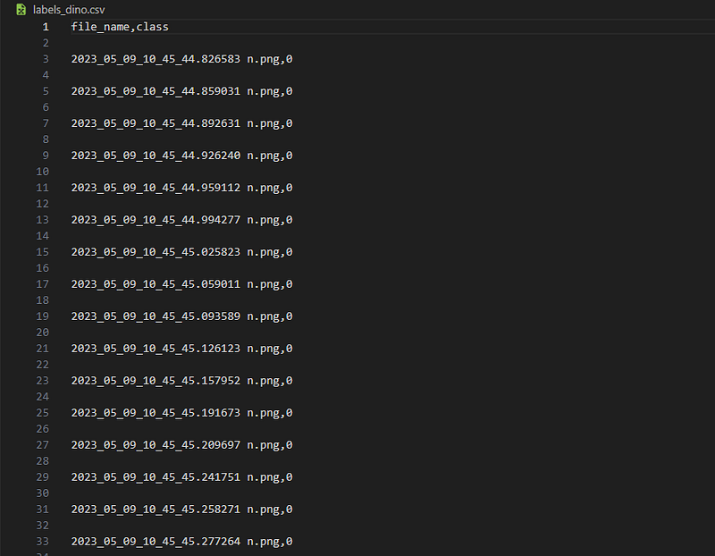
Finally, we use the csv module to write the labels to a CSV file called labels_dino.csv. We define the field names for the CSV file and use the DictWriter method to write the labels to the file. We first write the header row with the field names, and then use the writerows method to write the labels for each image in the directory to the CSV file.

This is how the labels_dino CSV file should look:

Ahhh…. the fun part in AI.. making the model. But wait, we need to take a few steps before creating the model.

Step 3: Creating the Model

Ahhh…. the fun part in AI.. making the model. But wait, we need to take a few steps before creating the model.

Step 3.1. Creating custom DinoDataset

To create our model, we first need to create a custom Pytorch dataset. We will call this DinoDataset. Start by creating a new notebook train.ipynb.

Let's import all the dependencies:

from torch.utils.data import Dataset, DataLoader
import cv2
from PIL import Image
import pandas as pd
import torch
import os
from torchvision.transforms import CenterCrop, Resize, Compose, ToTensor, Normalize
import matplotlib.pyplot as plt
import pandas as pd
from sklearn.model_selection import train_test_split
import torchvision.models
import torch.optim as optim
from tqdm import tqdm
import gc
import numpy as np

Now, let’s create an image transformation pipeline that’s required for EfficientNet v2:

transformer = Compose([
    Resize((480,480)),
    CenterCrop(480),
    Normalize(mean =[0.485, 0.456, 0.406], std =[0.229, 0.224, 0.225] )
])

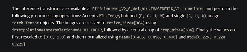
The values required are given in the PyTorch documentation of EfficientNet v2.

Now, let’s create our DinoDataset:

class DinoDataset(Dataset):
    def __init__(self, dataframe, root_dir, transform = None):
        """
        Args:
            csv_file (string): Path to the csv file with annotations.
            root_dir (string): Directory with all the images.
            transform (callable, optional): Optional transform to be applied
                on a sample.
        """

        self.key_frame = dataframe
        self.root_dir = root_dir
        self.transform = transform

    def __len__(self):
        return len(self.key_frame)
    
    def __getitem__(self, idx):
        if torch.is_tensor(idx):
            idx = idx.to_list()
    
        img_name = os.path.join(self.root_dir, self.key_frame.iloc[idx,0])
        image = Image.open(img_name)
        image = ToTensor()(image)
        label = torch.tensor(self.key_frame.iloc[idx, 1])

        if self.transform: 
            image = self.transform(image)

        return image, label

This is the definition of a custom dataset class DinoDataset, which inherits from the PyTorch Dataset class. It takes three arguments:

• dataframe: a pandas dataframe containing the filenames and labels for each image in the dataset.
• root_dir: the root directory where the images are stored.
• transform: an optional transform that can be applied to the images.

The __len__ method returns the length of the dataset, which is the number of images.

The __getitem__ method is responsible for loading the images and their corresponding labels. It takes an index idx as input and returns the image and its label. The image is loaded using PIL.Image.open, converted to a PyTorch tensor using ToTensor, and the label is read from the dataframe using iloc. If a transform is specified, it is applied to the image before it is returned.

Step 3.2. Creating Train and Test DataLoaders

key_frame = pd.read_csv("labels.csv") #importing the csv file with the labels of the key frames
train,test = train_test_split(key_frame, test_size = 0.2)  #splitting the data into train and test sets
train = pd.DataFrame(train) 
test = pd.DataFrame(test)

batch_size = 4
trainset = DinoDataset(root_dir = "captures", dataframe = train, transform = transformer)
trainloader = torch.utils.data.DataLoader(trainset, batch_size = batch_size) 

testset = DinoDataset(root_dir = "captures", dataframe = test, transform = transformer)
testloader = torch.utils.data.DataLoader(testset, batch_size = batch_size)

In this code, the train_test_split function from scikit-learn is used to split the dataset into training and testing sets with a 0.2 (20%) test size. The resulting splits are stored in the train and test variables as pandas DataFrames.

Next, a batch size of 4 is defined, and the DinoDataset class is used to create PyTorch DataLoader objects for the training and testing sets. The root_dir argument is set to "captures," which is the directory containing the captured images, and the transform argument is set to transformer which is the data preprocessing pipeline defined earlier. The resulting DataLoader objects are trainloader and testloader, which can be used to feed the data to the neural network during training and testing, respectively.

You can use higher batch_size values if you have access to a high-end GPU. For now, let us go with a smaller batch size.

Let’s check out the images in one of the batches in the dataloader.

dataiter = iter(trainloader)
images, labels = next(dataiter)

for i in range(len(images)):
        ax = plt.subplot(2, 4, i + 1)
        image = (images[i].permute(1,2,0)*255.0).cpu()
        ax.set_title(labels[i].item(), fontsize=20)  # Setting the title of the subplot
        ax.set_xticklabels([])   # Removing the x-axis labels
        ax.set_yticklabels([])   # Removing the y-axis labels
        plt.imshow(image)        # Plotting the image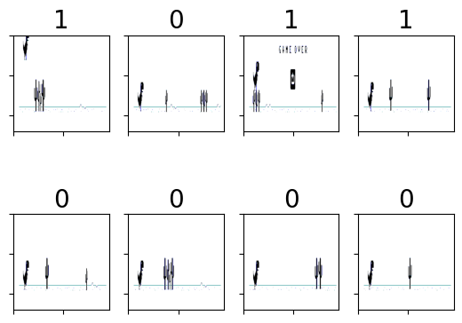

The number on top of each image shows the key that was pressed when that image was taken. 1 is for “space,” and 0 is for no key pressed.

Step 3.3. Creating the Model

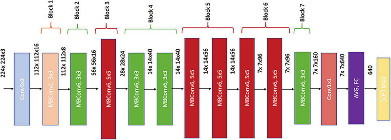
device = "cuda" if torch.cuda.is_available() else "cpu"
model = torchvision.models.efficientnet_v2_s()
model.classifier = torch.nn.Linear(in_features = 1280, out_features = 2)

model = model.to(device)
criterion = torch.nn.CrossEntropyLoss()
optimizer = optim.SGD(model.parameters(), lr=0.01, momentum=0.009)

This code initializes an EfficientNetV2-S model using PyTorch’s torchvision module and sets the number of output classes to 2. It then checks if a CUDA-enabled GPU is available and sets the device to “cuda” or “cpu” accordingly. The loss function used for training is Cross-Entropy Loss, and the optimizer used is Stochastic Gradient Descent (SGD) with a learning rate of 0.01 and momentum of 0.009.

EfficientNetV2-S is a variant of the EfficientNet architecture designed for mobile and embedded devices with limited computational resources. The output size of the last fully connected layer in the model is 1280, which is then fed into a linear layer with two output neurons representing the binary classification task.

Step 4: Training the Model

The choice of optimizer and hyperparameters like learning rate and momentum can have a significant impact on the performance of the model during training and should be tuned carefully to achieve the best results.

epochs = 15  # number of training passes over the mini batches
loss_container = [] # container to store the loss values after each epoch
for epoch in range(epochs):  # loop over the dataset multiple times

    running_loss = 0.0
    for data in tqdm(trainloader, position=0, leave=True):
        # get the inputs; data is a list of [inputs, labels]
        inputs, labels = data
        inputs = inputs.to(device)
        labels = labels.to(device)
        # zero the parameter gradients
        optimizer.zero_grad()

        # forward + backward + optimize
        outputs = model(inputs)
        loss = criterion(outputs, labels)
        loss.backward()
        optimizer.step()

        running_loss += loss.item()

    loss_container.append(running_loss)

    print(f'[{epoch + 1}] | loss: {running_loss / len(trainloader):.3f}')
    running_loss = 0.0

print('Finished Training')

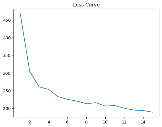
# plot the loss curve
plt.plot(np.linspace(1, epochs, epochs).astype(int), loss_container)

# clean up the gpu memory 
gc.collect()
torch.cuda.empty_cache()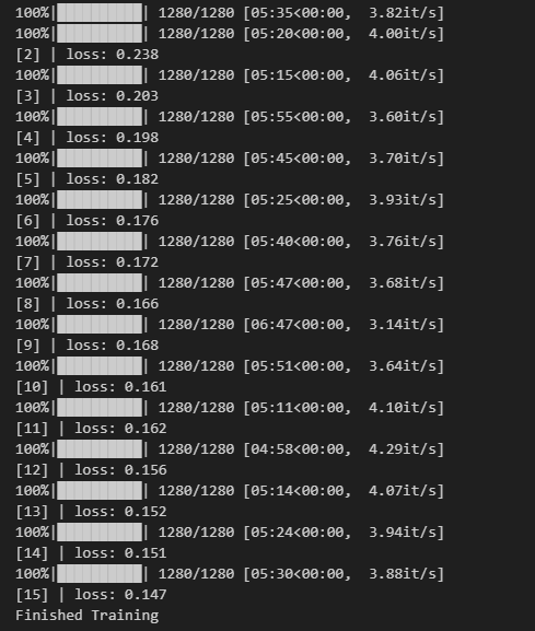

This is the training loop for the model. The for loop iterates over a fixed number of epochs (15 in this case), during which the model is trained on the dataset.

The inner for loop uses a DataLoader object to load the dataset in batches. In each iteration, the inputs and labels are loaded and sent to the device (GPU, if available). The optimizer's gradient is zeroed, and the forward pass is performed on the inputs. The model's output is then compared to the labels using the Cross-Entropy Loss criterion. The loss is backpropagated through the model, and the optimizer's step method is called to update the model's weights.

The loss is accumulated over the epoch to get the total loss. At the end of the epoch, the model is evaluated on the test set to check its performance on unseen data.

Note that tqdm is used to display a progress bar for each batch of data in the training loop.

This is what the loss curve looks like. We can keep running the training loop for more epochs.

We can also save our model using the following code:

PATH = 'efficientnet_s.pth'
torch.save(model.state_dict(), PATH)

Step 5: Testing the Model Performance

Let’s load a new EfficientNet Model that uses the weights we saved in the last step.

saved_model = torchvision.models.efficientnet_v2_s()
saved_model.classifier = torch.nn.Linear(in_features = 1280, out_features = 2)
saved_model.load_state_dict(torch.load(PATH))
saved_model = saved_model.to(device)
saved_mode = saved_model.eval()

correct = 0
total = 0
with torch.no_grad():
  for data in tqdm(testloader):
    images,labels = data
    images = images.to(device)
    labels = labels.to(device)

    outputs = saved_model(images)
    predicted = torch.softmax(outputs,dim = 1).argmax(dim = 1)
    total += labels.size(0)
    correct += (predicted == labels).sum().item()

print(f'\\n Accuracy of the network on the test images: {100 * correct // total} %')

This code evaluates the performance of the trained model on the test set.

The correct and total variables are initialized to 0, and then a loop over the test set is initiated. The testloader is used to load a batch of images and labels at a time.

Inside the loop, the images and labels are moved to the device specified during training (in this case, "cuda"). The saved model (trained earlier) is then used to predict the input images.

The torch.softmax() function is applied to the model outputs to convert them to probabilities, and then the argmax() function is used to determine the predicted class for each image. The number of correctly classified images is then calculated by comparing the predicted and true labels.

The total variable is incremented by the size of the current batch, and the correct variable is incremented by the number of correctly classified images in the batch.

After the loop completes, the percentage accuracy of the model on the test set is printed to the console. The accuracy for this model was 91% which is good enough to play the game. The hyperparameters for the optimizer can be tuned with more experimentation. There is still scope for improvement. In my future article, I will dive deeper into hyperparameter tuning using the weights and biases tool.

Step 6: Inferring / Playing the game

Create a new file dino.py. Run this file, come to the dino game screen, and watch your AI model play the game.

The first part of the code imports the necessary libraries and modules, including the EfficientNetV2-S model from the torchvision package, the keyboard library for simulating keyboard presses, the PIL library for image processing, numpy for numerical operations, and tqdm for progress tracking.

The code then loads the pre-trained EfficientNetV2-S model, adds a new linear classifier layer to it, and loads the trained weights of the new model from a saved checkpoint file. The model is then moved to the GPU for faster processing and set to evaluation mode.

The transformer variable defines a series of image preprocessing steps that are applied to the captured screen image before it is fed into the model. These steps include resizing the image to a square of size 480x480, cropping it to the center, and normalizing the pixel values using the mean and standard deviation of the ImageNet dataset.

The generator function is a simple loop that yields an empty value until the "esc" key is pressed.

The for loop continuously captures the screen image within a specified bounding box using the ImageGrab.grab() function. The captured image is then converted to a PyTorch tensor and moved to the GPU. The transformer is applied to the tensor to preprocess the image. Finally, the preprocessed image is fed into the model to obtain the predicted output probabilities. The torch.max() function is used to obtain the class label with the highest probability, and if the predicted label corresponds to the "jump" action, the keyboard.press_and_release() function is called to simulate a spacebar press, causing the character in the game to jump.

The loop continues until the “esc” key is pressed, and the process is tracked using the tqdm module. Your model should be able to play the dino game now. At least till the birds come.

I hope you had fun making this project and have learned a bit about general AI workflow for computer vision. For updates on new blogs and tutorials, follow me on Twitter and Linkedin.

Want to Connect?

Git Repostory
My website
LinkedIn
Twitter