How to Analyze A/B Test Results

A simple guide to using bootstrapping to analyze the results of A/B testing

When I was learning hypothesis testing, I got so overwhelmed by so many test statistics to choose from. Recently, I learned that bootstrapping can provide us an alternative to calculating p-value without having to worry about formulas! This article will guide you through the workflow of using Python and bootstrapping method for A/B testing results analysis.

Background

The dataset is from one of the projects in Udacity Data Analyst Nanodegree, which has the results of an e-commerce website A/B test. This A/B Test aims to test out if a new web page is better than the old one, and the main metric in this test is conversion rate, defined as the percentage of users who purchased this company’s product of all the users who visited the website. Our job is to determine if we should implement the new page or keep the old one.

Data Information

Let’s take a look at the dataset itself.

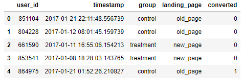
I want to focus on the analysis part, so I’ll not talk about data cleaning here. First, let’s calculate the probability of an individual converting regardless of the page they received.

convert_overall = df.converted.mean()
convert_overall

And it gives us 0.1206.

Now, let’s see how many users were assigned to control (old page) and treatment (new page) group, what their conversion rates are, and what the difference is.

size_old = sum(df.group == ‘control’)
control_convert = df.query(‘group == “control”’)[‘converted’].mean())

size_new = sum(df.group == ‘treatment’)
treatment_convert = df.query(‘group == “treatment”’)[‘converted’].mean())

print('There are {} users in the control group, and the conversion rate is {:.4f}.'.format(size_old, control_convert))

print('There are {} users in the treatment group, and the conversion rate is {:.4f}.'.format(size_new, treatment_convert))

print('The difference in conversion rate between control and treatment is {:.4f}.'.format(treatment_convert - control_convert))

There are 145,274 users in the control group, and the conversion rate is 0.1204. There are 145,310 users in the treatment group, and the conversion rate is 0.1208. The difference in conversion rate between control and treatment is 0.0004.

Hypothesis

Before we conduct our analysis, we need to define our null and alternative hypothesis first. Since our metric here is conversion rate, we can define our Null hypothesis as the new page will not change the conversion rate, and that is P(convert)ₙ = P(convert)ₒ, which equals to the convert_overall variable, 0.1206, as we calculated earlier. So, the Alternative hypothesis would be the new page brings us a different conversion rate than the old one does, in other words, they don’t come from the same population.

Confidence Level

The appropriate confidence level vary case by case, but here, we will use a 95% confidence level, which means we want to be 95% sure that the control and treatment come from the same population, and that their conversion rates are not different. As such, our p-value will be 0.05.

Bootstrapping

The idea of bootstrapping is using random sampling with replacement to perform inference about a population. There are 3 major steps to perform it.

Step 1: Make Bootstrapped datasets under the Null

We will simulate nₙ transactions with conversion rate of P(convert)ₙ and simulate nₒ transactions with conversion rate of P(convert)ₒ under the Null. Remember, in a perfect world where we have control over everything, if our Null Hypothesis is true, then we can expect the difference in conversion rate between old page (control) and new page (treatment) to be 0. So P(convert)ₙ = P(convert)ₒ = 0.1206 here.

new_page_converted = np.random.binomial(1, convert_overall, size_new)

old_page_converted = np.random.binomial(1, convert_overall, size_old)

Step 2: Calculate the difference

In this example, we will calculate the difference in mean of conversion rate between control and treatment groups.

new_page_converted.mean() - old_page_converted.mean()

Step 3: Repeat step 1 & 2 to form a distribution of the mean difference.

p_diffs = []
for _ in range(10000):
    sample_new = np.random.binomial(1, convert_overall, size_new)
    sample_old = np.random.binomial(1, convert_overall, size_old)
    sample_new_mean = sample_new.mean()
    sample_old_mean = sample_old.mean()
    p_diffs.append(sample_new_mean - sample_old_mean)

Let’s plot the difference distribution:

plt.hist(p_diffs);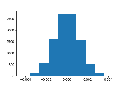

Calculate p-value

Remember, the observed difference between the conversion rate from old page and new page is 0.0004, and since the distribution here shows us what would happen if our Null hypothesis is true,

we can use it to calculate the p-value for observing a difference of 0.0004 or something more extreme, where more extreme means further from the null hypothesis than the observed difference, which in this case, means further than 0.0004 or -0.0004 from 0.

So, the p-value for the observed diff, 0.0004, is the probability of observing a boostrapped diff >= 0.0004 plus the probability of observing a bootstrapped diff <= -0.0004.

np.logical_or(np.array(p_diffs) >= obs_diff, np.array(p_diffs) <= -obs_diff).mean()

The result is 0.769. Because 0.769 > 0.05, we fail to reject the null hypothesis.

Lastly

Since p-value is way larger than 0.05, we cannot say that the new page will give us a higher conversion rate here. In real life, we not only need to analyze if the difference is significant, but also need to look at if the difference is practically significant, which means we would need to think about if the values it brings us surpasses the investment and losses.

In this analysis, I did not use test statistics to determine if I should reject Null hypothesis or not. The good thing about using bootstrapping is that I don’t need to assume the distribution of the data, or consider if the sample size is large enough.

Thanks to StatQuest’s videos which made writing this piece much easier!

Let me know what you think about this method!

Your support will mean so much to me and all the other writers here!