How to add Exponential Moving Averages to Your Trading Arsenal

Step-by-step examples using Python

Moving average indicators are used in a variety of trading strategies to spot long-term trends in the price data. One potential drawback of simple moving average strategies is that they weight all of the prices equally, whereas you might want more recent prices to take on a greater importance. The exponential moving average (EMA) is one way to accomplish this.

TL;DR

We walk through the EMA calculation with code examples and compare it to the SMA.

Calculating the Exponential Moving Average

The EMA gives more weight to the most recent prices via a weighting multiplier. This multiplier is applied to the last price so that it accounts for a larger chunk of the moving average than the other data points.

The EMA is calculated by taking the most recent price (we’ll call it 𝑃𝑡, or “price at time 𝑡”) and subtracting the EMA from the previous time period (𝐸𝑀𝐴𝑡−1). This difference is weighted by the number of time periods you set your EMA to (𝑁) and added back to the 𝐸𝑀𝐴𝑡−1.

Mathematically, we can write it like this:

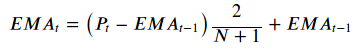
You may have noticed that the above equation has a slight problem, how does it get started? It’s referencing the last period’s EMA, so if you go to the first calculation, what is it referencing? This is usually alleviated by substituting the simple moving average (SMA) to initialize the calculation so that you can build the EMA for all time periods after the first.

Let’s show how this works with a simple example in Python by importing our packages.

import numpy as np
import pandas as pd
import yfinance as yf
import matplotlib.pyplot as plt

From here, we will build two functions to work together and calculate our indicator. The first function will be a simple implementation of the formula we outlined above:

def _calcEMA(P, last_ema, N):
    return (P - last_ema) * (2 / (N + 1)) + last_ema

The second function will calculate the EMA for all of our data, first by initializing it with the SMA, then iterating over our data to update each subsequent entry with the value in our SMA column or calling the _calcEMA function we defined above for rows greater than N.

def calcEMA(data, N):
    # Initialize series
    data['SMA_' + str(N)] = data['Close'].rolling(N).mean()
    ema = np.zeros(len(data))
    for i, _row in enumerate(data.iterrows()):
        row = _row[1]
        if i < N:
            ema[i] += row['SMA_' + str(N)]
        else:
            ema[i] += _calcEMA(row['Close'], ema[i-1], N)

    data['EMA_' + str(N)] = ema.copy()
    return data

Now, let’s get some data and see how this works. We’ll pull a shorter time period than we would use for a backtest and compare 10, 50, and 100 days of the EMA and SMA.

ticker = 'GM'
yfObj = yf.Ticker(ticker)
data = yfObj.history(ticker, start='2018-01-01', end='2020-12-31')

N = [10, 50, 100]
_ = [calcEMA(data, n) for n in N]

colors = plt.rcParams['axes.prop_cycle'].by_key()['color']

fig, ax = plt.subplots(figsize=(18, 8))
ax.plot(data['Close'], label='Close')
for i, n in enumerate(N, 1):
    ax.plot(data[f'EMA_{n}'], label=f'EMA-{n}', color=colors[i])
    ax.plot(data[f'SMA_{n}'], label=f'SMA-{n}', color=colors[i],
        linestyle=':')

ax.legend()
ax.set_title(f'EMA and Closing Price Comparison for {ticker}')
plt.show()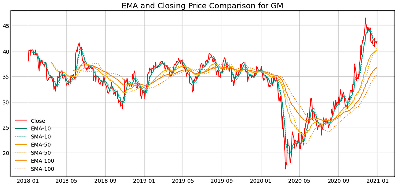

You can see in the plot above that the EMAs are more responsive to recent changes than the SMAs. Shorter time horizons too are even more responsive than longer time horizons which have a price “memory” that may stretch back months or more.

Moving averages of all types are lagging indicators meaning they only tell you what has already happened in the price. However, this doesn’t mean they can’t be useful for identifying trends and developing strategies that use one or more moving average indicators.

One common approach is to use moving averages to look for cross-overs — points where a faster indicator moves above or below a slower indicator to generate signals. Another possibility includes using these indicators as market level filters to adjust risk exposure.

If you have an idea, go ahead and test it out, see how EMA, SMA, and other values can be combined to develop new and profitable trading strategies.

At Raposa, you can quickly test your ideas with no code and high-quality data to run backtests. Find a strategy that works for you and deploy it to get live trading alerts.