
Python for Traders — Storytime
How I Used Mathematics and AI to Increase my Profits by 22.4% — Part2
A walk-through of a misknown machine learning algorithm used by Netflix to trade like a high-frequency trader.

This article is the second part of this A to Z tutorial on how to use machine learning and AI to develop a trading model.
Today, in this article, we will cover the second part of the article on how to use math to boost your trading performances. Part 2/3
This model is adapted for day trading but can be used by anyone and for different purposes. Either for building a portfolio of data science projects before going to an interview, understanding the mathematical intuition behind AI, or launching a career in Finance.
FYI — You can access the first part following this link:
Let’s start!
In the previous article …
In the previous article, we started by covering the classification algorithms (used by Netflix) and how to use them for trading purposes.
Then we have defined our roadmap to develop our machine learning model for day trading:
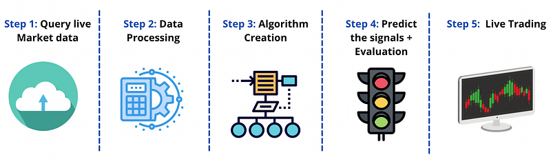
We have defined a way to get live market data using yahoo finance API, and we chose an interval of one minute to stay in our day trading window.
Then we refined the second step into four distinct stages:
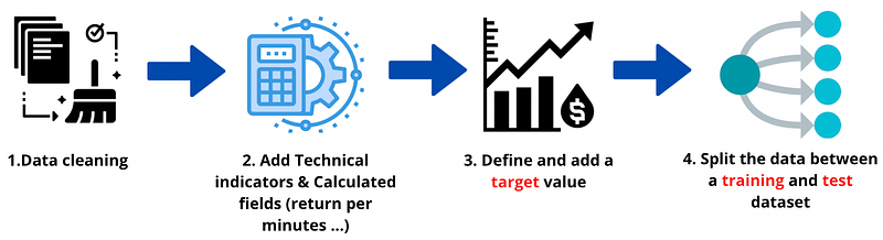
We started by cleaning the variable that can lead to default our model (everyone must clean this variable before starting developing a model). And calculate the RSI for each minute.
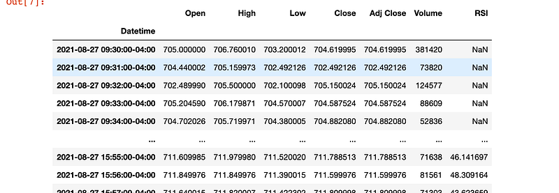
And here how is looking the data frame at the end of the first part:
We ended by visualising these data and found an exciting correlation between RSI and market movement:
Now that we have covered what we have seen so far, we can continue enhancing our model.
Add trending indicators to help the machine.
Before starting indexing our values in percentage of change, we will add three different trading indicators to give more information about market trends and market volatility.
The indicators that we will add are moving averages called MACD by traders, parabolic SAR to determine trend direction and potential reversals in price and the average directional index (ADX) to determine the strength of our trends.
Similarly to what we did for the RSI, we use the Talib library to calculate these fields.
On top of these trading indicators, we have added the correlation coefficient between the SMA and the market to get more information.
That must recall a lot of good memories to everyone who studied finance at university :) Usually, finance teachers call it the beta coefficient.
Mr Chavez (my finance teacher at uni) must be proud of me :)
So, joke aside. Now that we added the most influential trading indicators, we can pursue extra information to make the model more robust.
Previous minutes values
The last variable that I will recommend adding, and it is just based on my own experience, is to pass the previous minute’s `High`, `Low`, and `Open` prices as input to the algorithm. This will help the algorithm sense the volatility of the past time period.
Very easy to do with the shift function already included in python:
And here we go; we just added three more variables.
We will also create two more columns as features: the change in `Open` prices between last-minute and current minute & the difference between current minute’s `Open` and last minute’s `Close` prices.
And before going further and start implementing the algorithm, we will add the percentage of change that will help us detect a bear to a bull period. Indeed a percentage of change will be more beneficial for the algorithm to judge the movement. And it will permit us to segregate our values between high profitable period vs range period vs loss period.
As shown below:
Calculate the return
So, let’s calculate the returns (mathematically speaking, the percentage of change evocated above) for every data point(rows). We also save returns of past n minutes in n columns named as return1, return2 and so on. This will help the algorithm to understand the trend of the returns in the last n periods.
Before ending the data process, the last cleaning step is required for the correlation column before setting our output (as described in the diagram above) and split up the data.
Cleaning correlation column
I noticed that a correlation coefficient over 1 and below -1 sometimes appears because of missing values. We will change all values less than -1 to -1 and all values greater than 1 to 1.
This doesn’t affect our calculations because the extreme values are realised due to NaN values in the data, which need to be handled before training the algorithm. Then we drop all NaNs from the entire data frame.
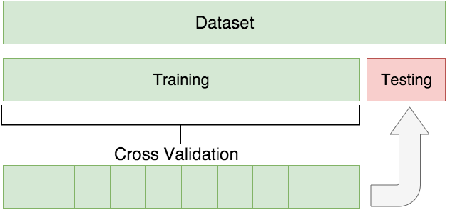
Now that we have cleaned/trimmed our variables and added our calculated fields, we will need two data structuring/processing steps before implementing our machine learning algorithm.
We first divide our dataset between a training and testing set, then set up the target values for the training dataset.
Here is an example of how to structure the data:
Everything is explained beautifully within this article about the importance of this step for an AI and ML model:
Now that we have understood the importance and the difference between training and a test dataset, we will create a split function to replicate this structure.
Split function
We will be using 80% of the data to train and the rest 20% to test. We will create a split parameter that will divide the data frame in an 80–20 ratio.
The proportion to be divided is entirely up to you and the task you face. It is not essential that 80% of the data be for training and the rest for testing.
For instance, if you have a dataset with over 10,000 rows, using a split of 95–5 ratio would be better.
This can be changed as per your choice, but it is advisable to give at least 70% data as train data for good results. But in this case, I would recommend 80% because we will have enough data to train the model and enough data to validate the test.
So, let’s create a “split” function that will catch 80% of the dataset.
For now, this variable is just getting the value of 80% of the total number of rows as an integer. We will use it in the future to determine the last row to take into consideration.
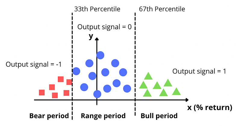
Now it is time to define our output signal (also called target).
Define output signal
The output signal will be based on the percentage return and split into three categories:
- Bear period: Output signal = -1
- Range period: Output signal = 0
- Bull period: Output signal = 1
So let’s execute our lines of code:
And here we go, we assign our output value to the column created called signal.
And we will end this first step by creating the features and values.
Drop unnecessary variables
We will drop the columns `Close`, `Signal`, `Time`, `High`, `Low`, `Volume`, and `Ret` since the algorithm will not be trained on these features. Next, we assign `Signal` to `y`, which is the output variable you will predict using test data.
At this moment, we have split our dataset into two distinct parts. The first one will contain the trend of the share and the final output. And a second one where we will evaluate our model.
Now the dataset is ready to propel and start our live trading.
Now that we have our training set, it is time to find our best parameters. In the next part, we are going to step up again in terms of algorithm deployment.
How to create machine learning from A to Z will be discussed in the third and last parts. The third part will be published on Wednesday, 22nd September 2021. So, think to subscribe on Medium or Youtube to get the update.
I love you all. I hope you like this second part; the third part will be even more exciting.
In the following article …
In the third part, we will develop our machine learning and run our AI robot for trading!
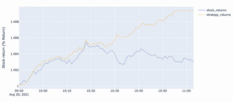
Below, you can get a sample of the final results:
You can access the full video tutorial below, with further explanations if you want to develop it at home:
Happy coding,
Sajid


