
How does the strategy of a football team evolve over a match?
Inferring and Evaluating Team Strategy in Football Using Automated Formation Analysis of Tracking Data
The paper discussed in this article presents a new technique for measuring, classifying, and analyzing team formations in professional football matches using a large sample of player tracking data. The method involves hierarchical agglomerative clustering, which identifies the unique set of offensive and defensive formations used by teams. The authors use Bayesian model selection criteria to classify new formation observations, creating tactical summaries of each match. They also examine how formation choices relate to playing style and discuss potential applications of their methodology.
The authors are Laurie Shaw (Harvard Data Science Initiative and Harvard Sports Analytics Lab) and Mark Glickman (Harvard Sports Analytics Lab and Harvard Department of Statistics).
Introduction
The paper first highlights the importance of team formations in football and the role they play in team strategy. While formations are central to the selection of player roles and playing style, descriptions of formations are largely reliant on classifications based on the number of defenders, midfielders, and forwards. This is a crude summary that overlooks the fluid and nuanced player configurations that are dependent on the game state. Previous studies have assumed that formations remain static throughout a match, which precludes analysis of how in-match tactical changes affect the outcome.
To address this limitation, the authors present a new, data-driven technique for measuring and classifying team formations as a function of game state. The technique analyses the offensive and defensive configurations of each team separately and dynamically detects major tactical changes during the course of a match. The authors use unsupervised machine learning techniques to identify the unique set of template formations used by the teams in the dataset. They classify individual formation observations in a larger sample of matches according to these templates to study transitions between defence and attack and analyse changes in formation during matches. Finally, the authors discuss the practical applications of their methodology.
Methodology
The methodology section of the paper outlines the three key stages of the authors’ new technique for measuring and classifying team formations. The first stage involves a new algorithm that measures team formations as a function of time during a match by averaging vectors between neighbouring players in local possession windows. The second stage involves identifying the unique offensive and defensive formations used by teams in a large training set of tracking data through agglomerative hierarchical clustering. In the third stage, the authors incorporate the set of identified formation clusters into a Bayesian model selection algorithm to dynamically classify formation observations and systematically detect formation changes during matches.
The tracking data used in the analysis consists of 180 matches from a single season of an elite professional league. The data for each match includes the positions of all 22 players and the ball, sampled at a frequency of 25Hz. Individual player identities are tagged in the data, enabling tracking of each player over time. Overall, the authors’ methodology involves using advanced statistical techniques and large datasets to develop a comprehensive and nuanced understanding of team formations in professional football.
Measuring team formations
In this section, the authors describe their algorithm for measuring team formations during a match. The algorithm calculates the vectors between each player and their teammates at successive instants during a match and then averages these vectors over a specified time interval to determine their designated relative positions. The authors use a pairwise approach to measure team formations, rather than measuring the average positions of each player in the center of mass frame of the team, as in previous studies.
The authors use tracking data from 180 matches from a single season of an elite professional league. They measure defensive and offensive formations separately by aggregating together consecutive possessions of the ball for each team into two-minute, non-contiguous time periods. They exclude possessions that last for less than five seconds and end the window if a substitution occurs. The authors obtain ten defensive and ten offensive formation observations for each team during a match.
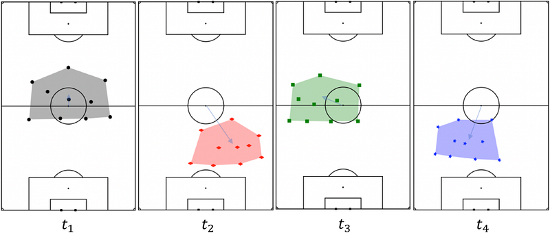
Figure 1 shows the positions of the defending team at four instants during the first half of a match, and it is clear that the players largely retain their relative positioning, maintaining a 4–3–3 formation.
The final spatial distribution of the outfield players is determined using an algorithm that identifies the relative positions of each player’s nearest neighbour until the positions of all players in the team have been determined. The centroid of the formation is set to be the position of the player in the densest part of the team, as determined by the average distance to the third-nearest neighbour.
The advantage of the pairwise approach to measuring team formations is that the location of a player in a formation is dictated solely by his position relative to his neighbouring teammates. This is in contrast to measuring the average positions of each player in the centre of mass frame of the team, which would result in the formation positions being influenced by every other player on the team.
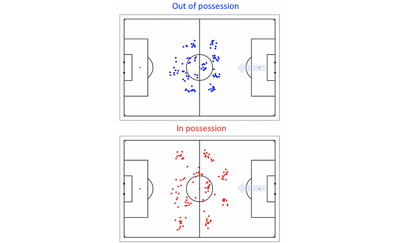
Figure 2 presents four examples of individual formation observations.
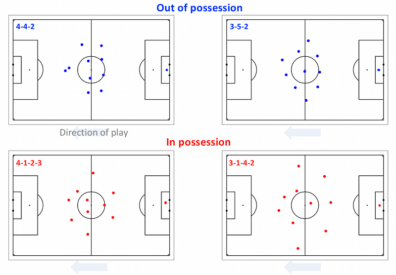
Next, the authors discuss the formation observations for one team during a single match, as shown in Figure 3. The upper plot shows the team’s formation when they were out of possession, which was a 4–1–4–1 formation with a single defensive central midfielder and a lone striker. The lower plot shows the team’s formation when they were in possession, with the outside midfielders advancing to form a front three and the full backs moving level with the defensive midfielder. The right central midfielder played slightly deeper than the left central midfielder, which introduced a small asymmetry to the team when attacking.
The relative positions of the defensive players in the team were well constrained, but the position of the offensive players, particularly the central striker, was much more broadly distributed, both in and out of possession. Additionally, the area encompassed by the outfield players (the convex hull) when attacking was twice the area when they were defending.
The observations were consistent, indicating that the manager did not make a significant formation change during the match. This information is useful for understanding how a team plays in different situations and can inform strategic decisions for future games.
Identifying unique formations
In this section, the authors describe how they identify unique formations using agglomerative hierarchical clustering. They applied their methodology to a training sample of 100 matches and obtained 3976 observations of offensive and defensive formations. The remaining 80 matches were used as a test set for validation.
To quantify the similarity of two formation observations, the authors used the Wasserstein distance, which is a solution to the optimal transport problem. Each observation is a set of 10 bivariate normal distributions, one for each outfield player, where the mean of each distribution is the position of a player in the formation, and the covariance matrix is an estimation of how far the player deviated from his position during the two-minute possession window in which the formation was measured.
To find a pairing of the players in two formation observations that minimizes the square of the sum of the Wasserstein distances, the authors used an allocation matrix. Each row and column in the matrix must uniquely consist of nine 0s and a single 1. The authors used the Kuhn-Munkres algorithm to find the allocation matrix that minimizes the total cost.
To compare two formation observations, the authors introduced a variable scaling factor, k, that expands or contracts a formation around its centre of mass, scaling the player covariances accordingly. When comparing two formation observations, they searched for the value of k that minimised the Wasserstein distance between them. They used agglomerative hierarchical clustering with the Ward metric as a linkage criterion to identify 20 unique formation templates or clusters used by the teams in their training sample. The results are shown in Figure 4.
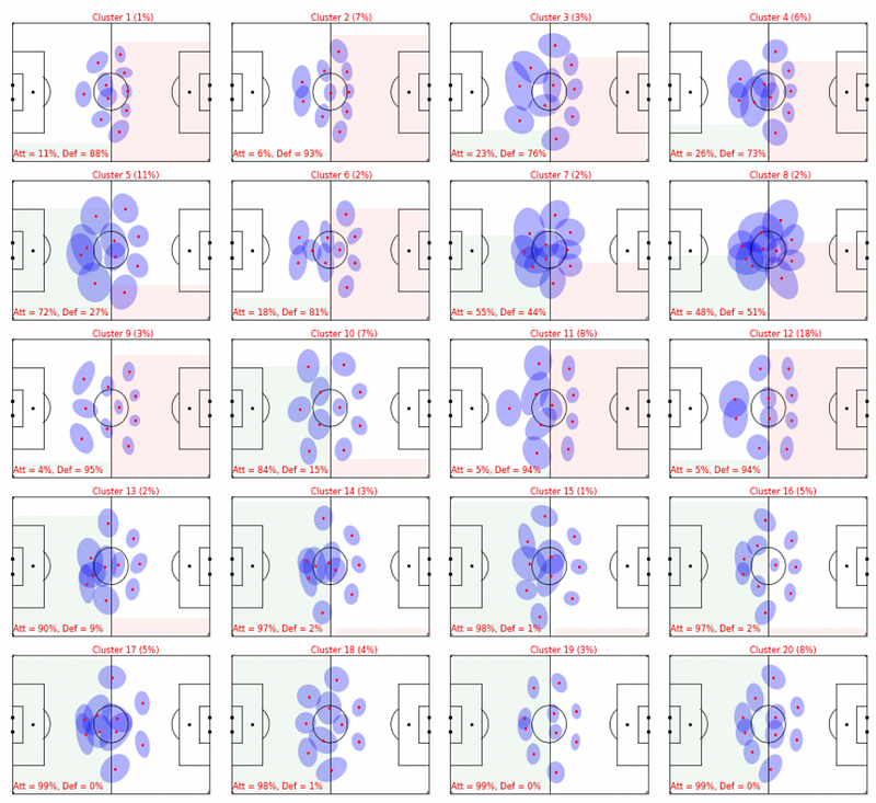
The authors then describe the results of their application of agglomerative hierarchical clustering to the tracking data from their training sample of 100 matches. The aim was to group similar observations of offensive and defensive formations and identify the unique formation types adopted by the teams during the matches.
The results of the agglomerative hierarchical clustering showed a clear ordering of the clusters that highlighted the difference between defensive and offensive formations, which was lost in previous analyses of formations in football. The top row in Figure 4 contains formation clusters with five defenders and variations in the number of midfielders and forwards, which predominantly consist of defensive formation observations. The following two rows indicate variants of a back four, which contain a mix of attacking and defensive formation observations. The fourth and fifth rows contain clusters that almost entirely consist of offensive formation observations.
Overall, the hierarchical clustering efficiently separated observations of defensive and offensive formations, even though it could not use the differences in their scale size (or area encompassed) as a discriminator because of the application of the scaling factor, k.
Formation classification
In this last section, the authors describe the final step of their methodology, which is a Bayesian model selection algorithm used to estimate the probability that a newly observed formation belongs to each of the 20 formation clusters identified in the previous section. The probability is calculated by comparing the position and covariance matrix of each player in the formation observation to those in each of the 20 clusters. The scaling factor, k, is also used to account for variations in the size of the formation.
To assign each player in a formation observation to a specific role in a cluster, the authors use the Kuhn-Munkres algorithm, as described in the previous section. This allows them to identify the maximum probability cluster for each formation observation, which enables them to classify formation observations throughout a match and detect tactical changes in real-time.
By dynamically detecting tactical changes, the methodology allows for a more nuanced understanding of how teams adapt and respond to changing match conditions. This information can be used by coaches and analysts to inform strategy and improve performance.
Results and analysis
In this section, the paper discusses the results and analysis of their formation detection and classification scheme on a full sample of 180 matches.
Transitions
The researchers investigate transitions between defense and offense by identifying the most frequently paired defensive and offensive formation clusters. They use a Sankey diagram to visualize these pairings, with the left-hand side showing defensive formation clusters and the right-hand side showing offensive formation clusters, and links indicating the formations that were typically employed together as teams gained and lost possession.
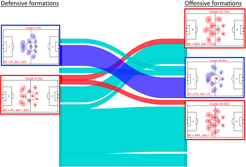
The diagram shows the connections between formations that were typically employed together as teams gained and lost possession. Two examples are highlighted, showing how teams transition between formations when gaining possession. The examples show that the defensive and offensive formation pairings are consistent and that some defensive configurations provide more flexibility in terms of different attacking options than others.
Strategic summaries and changes in formations
In this section of the paper, the authors discuss the strategic summaries and changes in formations enabled by their methodology. They present Figure 6, which charts the defensive and offensive formations during a match between two teams (Red team and Blue team) throughout the course of the match. The circles indicate the offensive formation observations of each team, while the diamonds indicate the defensive formations. Goals and substitutions are also indicated in the chart. The authors analyze the chart and point out that the Red team made a significant change in formation, switching from a 3–4–3 formation to a 4–3–3, which resulted in them scoring shortly after half time, but ultimately losing the match 2–1.
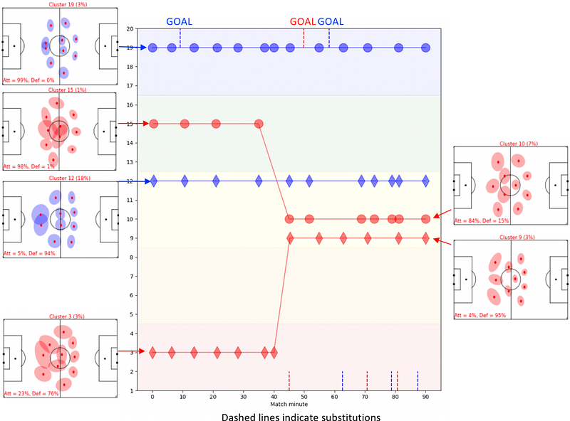
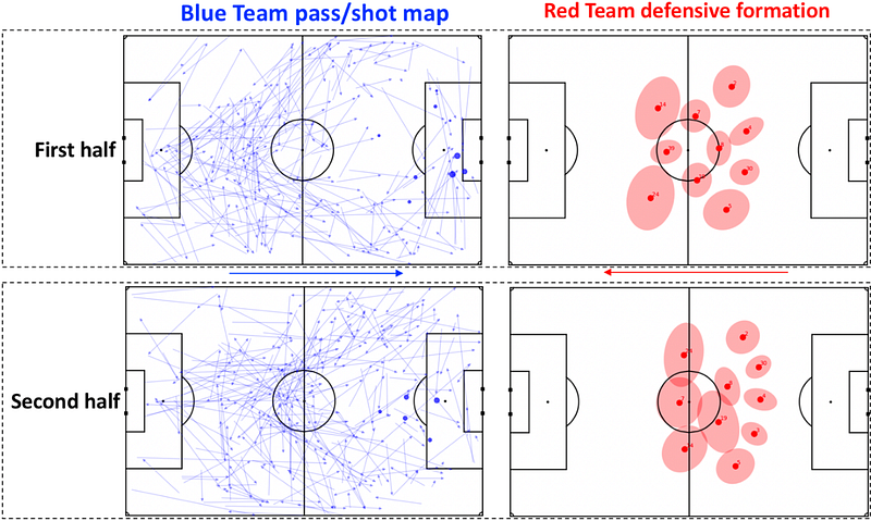
Following this, the paper describes how automated detection of formation changes, combined with event data, enables the investigation of why certain tactical changes were made and evaluation of the impact they had on the outcome of a match. The authors provide an example where the Red team switched from a 4–3–3 to a 5-man defense in the second half of the game to prevent the Blue team from creating chances from their right side. The pass map for the second half indicated that the change in formation was effective in preventing the Blue team from creating chances from their right side, with the focus of their passing switching more towards the center and left of the pitch.
Practical applications
The paper concludes by discussing the practical applications of the proposed methodology for tracking data in football analysis. Firstly, it enables teams to study the opposition’s habitual response to specific match situations and anticipate and exploit their tactical changes. Secondly, it enables the detailed investigation of factors that disrupt the defensive formation of a team and relate them to chance creation. Finally, the methodology can be extended to consider formations in more specific phases of possessions, such as transition, establishment, progression, and chance creation, and incorporate player velocity information to identify and understand marking systems and high press operations.
References
- Shaw, L., & Glickman, M. (2019). Dynamic analysis of team strategy in professional football. Barça sports analytics summit, 13. https://static1.squarespace.com/static/5b048119f2e6b103db959419/t/5dd45c9b0c0fd15052cb7335/1574198467133/Dynamic+analysis+of+team+strategy+in+professional+football+By+Laurie+Shaw+And+Mark+Glickman.pdf