
How Boosted Trees Inference Works

The gradient-boosted trees is a popular machine-learning model widely used across all industries. Thus, understanding how boosted tree inference works is crucial if you want to serve the model in low latency, high throughput environment.
What is the gradient-boosted trees model?
In this article, I will not discuss how gradient-boosted trees training works. Instead, I will focus on how the gradient-booted trees model produces predictions. For more information on how gradient-boosted trees works, you can refer to XGBoost documentation.
Boosted trees inference
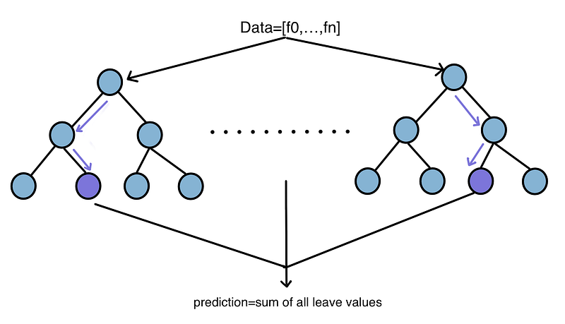
Boosted trees inference is the same as random forest; the difference only arises from how we train them. Specifically, it aggregates the score from all trees to make predictions, which we call tree ensembles. The leaves from each tree contain prediction values. Each tree will reach a different leaf value depending on the dataset:
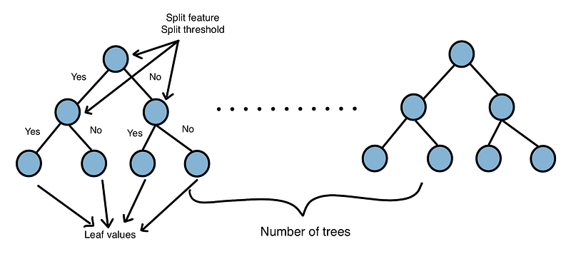
Each node in a tree will define the feature it will use to make a decision and a threshold according to that value. If the value of that feature is below the node threshold, it will go to the left, else go to the right:
If the training objective is regression, then the prediction is just the sum of all reached leave values:

However, if the objective is binary classification, the final prediction will go through an additional sigmoid function to produce probability prediction:

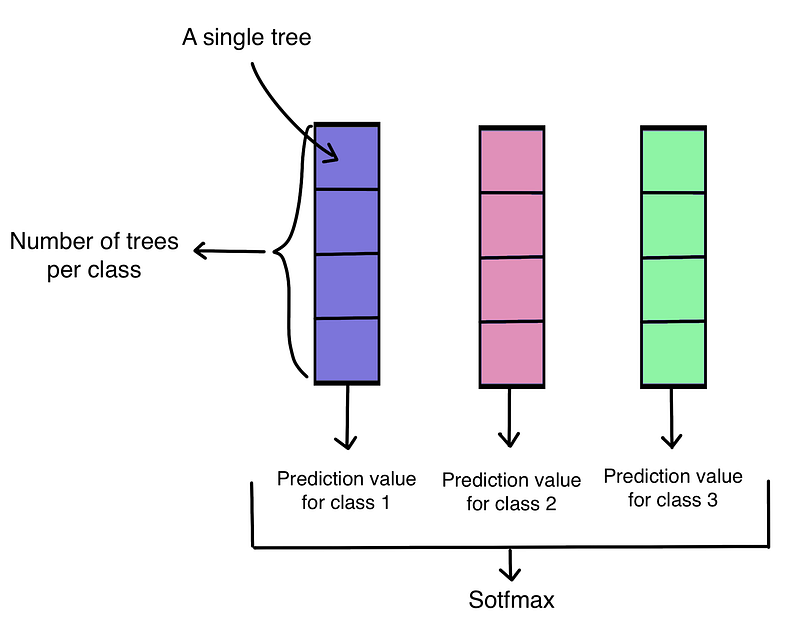
For a multi-class objective, gradient-boosted trees will train for each class separately. Each class will generate a prediction value using a mechanism similar to binary classification. Finally, it will convert all these prediction values into probabilities using softmax:
Understand XGBoost inference
DMLC XGBoost is a popular gradient-boosting library which many companies adopt. Understanding the XGBoost export model file is useful if we want extra flexibility to serve our models. Some additional flexibility we can have are:
- Writing the serving method in our preferred language (C++, Golang, …)
- Add additional parameters to the model file according to our needs.
To serve the XGBoost model, we need to train it first. Here, I will use sklearn built-in breast cancer dataset for training:
import numpy as np
import xgboost as xgb
from sklearn import datasets
from sklearn.datasets import dump_svmlight_file
from sklearn.model_selection import train_test_split

X, y = datasets.load_breast_cancer(return_X_y=True)
X_train, X_test, y_train, y_test = train_test_split(X, y, test_size=0.2, random_state=0)

# For binary classification.
dtrain = xgb.DMatrix(X_train, label=y_train)
classification_param = {'max_depth': 4, 'eta': 1, 'objective': 'binary:logistic', 'nthread': 4, 'eval_metric': 'auc'}

num_round = 10
bst = xgb.train(classification_param, dtrain, num_round)
y_pred = bst.predict(xgb.DMatrix(X_test))

np.savetxt('../data/breast_cancer_xgboost_true_prediction.txt', y_pred, delimiter='\t')
dump_svmlight_file(X_test, y_test, '../data/breast_cancer_test.libsvm')
bst.dump_model('../data/breast_cancer_xgboost_dump.json', dump_format='json')Note: This code is only tested with xgboost version 1.2.0
num_round is the total number of trees, and max_depth is the maximum depth each tree can have. The export model file will look like this:
We can see that the export model file is a JSON file with the following structure:
type xgboostJSON struct {
 NodeID                int            `json:"nodeid,omitempty"`
 SplitFeatureID        string         `json:"split,omitempty"`
 SplitFeatureThreshold float64        `json:"split_condition,omitempty"`
 YesID                 int            `json:"yes,omitempty"`
 NoID                  int            `json:"no,omitempty"`
 MissingID             int            `json:"missing,omitempty"`
 LeafValue             float64        `json:"leaf,omitempty"`
 Children              []*xgboostJSON `json:"children,omitempty"`
}
Here are the parameter descriptions:
- nodeid: The node id for identifying which nodes the model should go to.
- split: The feature that the model uses for making the decision.
- split_condition: The threshold used for making a decision. If the split feature has a value smaller than the split condition, the model will go to the yes node or the no node.
- yes: The node id that the model should go to if the feature value is smaller than the split condition.
- no: The node id that the model should go to if the feature is larger or equal to the split condition.
- missing: The node id that the model should go to if the feature is missing.
- leaf: If the node is a leaf, it will contain a float value or be empty.
- children: Contains children values or empty if the node is a leaf.
XGBoost inference libraries
Once we fully understand the XGBoost JSON model structure, implementing the inference logic with our preferred language is trivial. We can significantly reduce the latency of the serving model if we directly integrate our model in our native backend language. If you are using Golang as your backend logic, here are some libraries you can use:
- https://github.com/dmitryikh/leaves
- https://github.com/Elvenson/xgboost-go (My implementation which supports XGBoost dump_model API)
I hope you find this post useful :). Thanks for reading til the end.


