How Bayesian statistics convinced me to hit the gym

A fun journey into the theory of Linear Regression with a Bayesian touch (and yes, I use metric measurements in this post)

As the title of the article suggested, I will make a scientific investigation into my physique.

“ C’mon, you can’t be serious !!!”

Yes I am. So a little bit of background information: I originally come from Vietnam, went to high school in Singapore and currently attend college in USA. I often heard people making fun of how small I look, how underweight I must be and how I should do exercise, hit the gym and gain weight in order to have “a nicer physique”. I often took these comments with a pinch of salt. For somebody who is 1m69 (5'6) in height and 58kg (127lb) in weight, I have close-to-perfect BMI index (20.3).

“No dude! We are talking about the PHYSIQUE”

Ok, I get it, nobody is talking about BMI here.

Thinking about it, people may have a good point: given that I am slightly taller and have the exact same weight as an average Vietnamese male (a Wikipedia profile of 1m62 and 58kg), I may “look” a little skinnier. Look is the key word here. The logic is quite simple, isn’t it? If you stretch yourself a little bit and have the same exact weight, you should look, well, leaner and skinnier. I consider this an actually serious scientific question to investigate further:

How small I am (in weight) for a Vietnamese male of 1m69 in height?

We need a methodological way to investigate into this topic. A good way to go forward is to find as much data of Vietnamese men’s height and weight as possible and see where I stand among them.

The Vietnamese population profile

After browsing through the web, I found out a survey research data¹ that contains demographic information of more than 10,000 Vietnamese people. I limited the sample size to Male of the age group 18–29. This allows me to have a sample size of 383 Vietnamese males whose age are around 18–29, which is probably good enough for analysis.

At first, let’s plot the weight of the population and see how I would fit in among the young Vietnamese men.

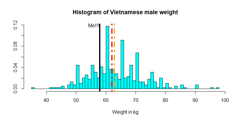
The red line shows the median of the sample while the orange line shows the mean

This plot suggests that I am slightly below both the average and median weights of those 383 Vietnamese young men. Encouraging news? Kind of but not quite. See, the question is not really about how my weight compares to those in this sample per se, but given the height of 1m68, what can we infer about my weight compared to the entire Vietnamese population, assuming that the Vietnamese male population is well-represented by these 383 individuals? To do this, we need to dive into a regression analysis.

At first, let’s plot a 2-dimensional scatter plot of heights and weights

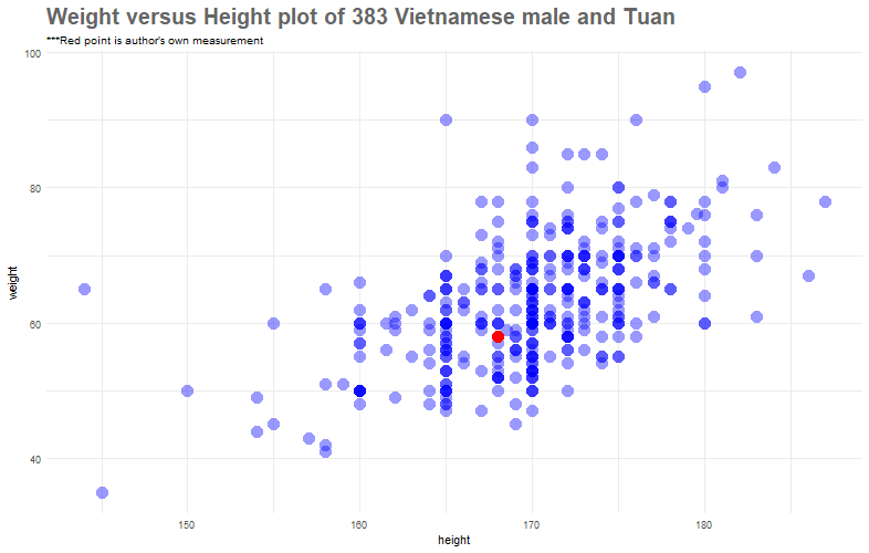
Well, I just look average. In actual fact, if we only look at the data of those who are 168cm in height (imagine a verticle line that goes at 168cm and passes through the red point), I sort of weight a little bit less than these people.

Another important observation is that the plot suggest a positive linear relationship between the height and weight of Vietnamese male. We will do a quantitative analysis to get to the bottom of this relationship.

First, let’s quickly add a standard“ ordinary least square” line.

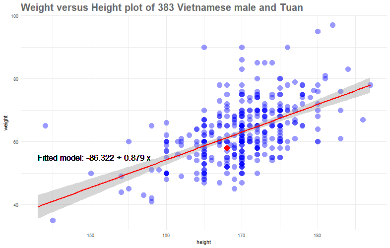
We could interpret our least-squares line y=−86.32+0.889x as suggesting that for a usual profile of a Vietnamese male at my age, an increase in 1 cm of height would observe an increase in weight of 0.88kg.

However, this still does not answer our question; that is, given somebody of my height (1m68), is 58kg considered too much, too little or just about average? To rephrase this question in a more quantitative manner, if we have a distribution of all of those who are 1m68 in height, what is the chance of my weight falls into the 25, 50 or 75-percentile? To do this, let’s dig deeper and try to understand the theory behind Regression.

The theory of Linear Regression:

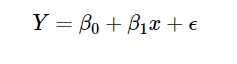
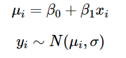
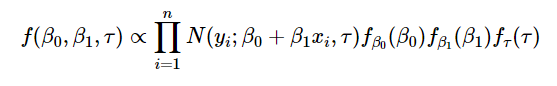
In a linear regression model, the expected value of the Y variable (in our case, the person’s weight) is a linear function of x (height). Let’s call the intercept and slope of this linear relationship β0 and β1; that is, we assume that E(Y|X=x)=β0+β1× x. We do not know β0 and β1 so we treat them as unknown parameters.

In the most standard linear regression models, we further assume that the conditional distribution of Y given X=x is Normally distributed

This means that simple linear regression model:

can be rewritten as:

Note that in many models, we can replace variance parameter σ with precision parameter τ, where τ=1/σ.

To summarize: dependent variable Y follows normal distribution parameterized by mean μi and by precision parameter τ. μi is a linear function of X parameterized by β0 and β1

Finally, we also assume that the unknown variance does not depend on x; this assumption is called homoscedasticity.

That’s a lot, but you can visualize what I have discussed with this image.

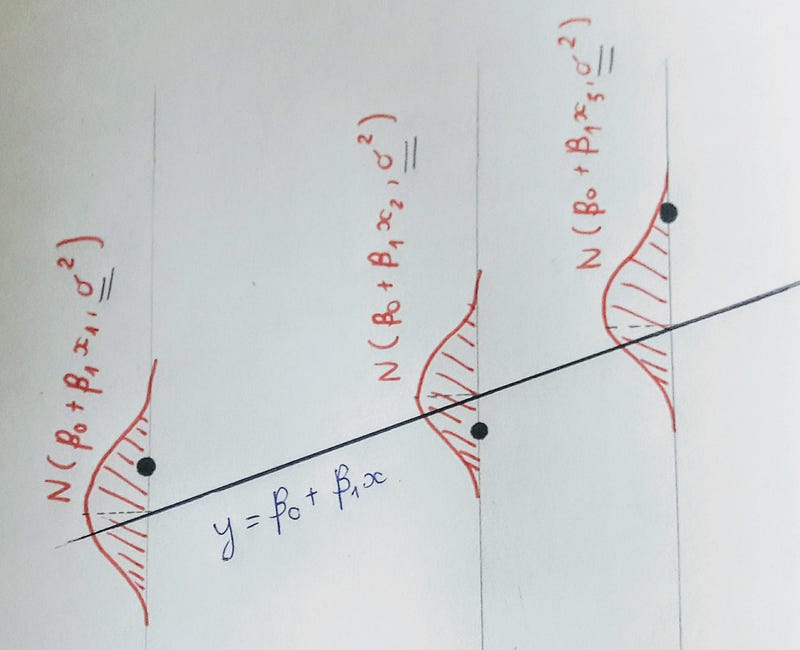
In an actual data analysis problem, all we are given is the black dots — the data. Notice how the normal distribution around each dots look exactly identical. This is the essence of homoscedasticity .Using the data, our goal is to make inferences about the things we don’t know including β0, β1 (which determine the mysterious black line) and σ (which determines the width of the red Normal densities from which the y data values are drawn).

Estimating parameters

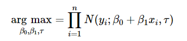
Now, there are a couple of ways you can do to estimate β0 and β1.If you estimate such model using ordinary least squares, you do not have to worry about the probabilistic formulation, because you are searching for optimal values of β0 and β1 by minimizing the squared errors of fitted values to predicted values. On another hand, you could estimate such model using maximum likelihood estimation, where you would be looking for optimal values of parameters by maximizing the likelihood function

Note: an interesting result (not demonstrated mathematically here) is that if we make the further assumption that the errors also belong to a normal distribution the least squares estimators are also the maximum likelihood estimators.

Linear Regression with a Bayesian touch:

The Bayesian approach, instead of maximizing the likelihood function alone, would assume prior distributions for the parameters and use Bayes theorem:

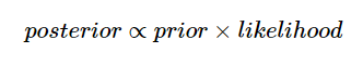
The likelihood function is the same as above, but what changes is that you assume some prior distributions for the estimated parameters β0, β1, τ and include them into the equation:

“Wait, what is the deal with this prior gig and why does it make our formula look 10x more complicated?”

Believe me, this prior business feels kind of strange, but it is very intuitive. The truth is, there is a strong philosophical reasoning as to why we could assign an unknown parameters (in our case β0, β1, τ ) with some seemingly arbitrary distributions. These prior distributions are meant to capture our beliefs about the situation before seeing the data. After observing some data, we apply Bayes’ Rule to obtain a posterior distribution for these unknowns, which takes account of both the prior and the data. From this posterior distribution we can compute predictive distributions for future observations.

Repeat after me: These prior distributions are meant to capture our beliefs about the situation before seeing the data

The final estimate will depend on the information that comes from 1) your data and 2) your priors, but the more information is contained in your data, the less influential are priors.

“So I can choose whatever prior distribution?”

That is a good question, since there is unlimited number of choices. There is (in theory) just one correct prior, the one that captures your (subjective) prior beliefs. However, in practice, the choice of the prior distribution can be rather subjective and sometimes, arbitrary. We could just choose a Normal prior with a large standard deviation (small precision); for example, we could assume β0 and β1 come from a Normal distribution with mean 0 and SD 10,000 or whatever. This is called an uninformative prior because essentially this distribution will be rather flat (that is, it assign almost equal distribution to any value in a particular range).

What follows is that if this family of distributions is our choice, we do not need to worry about which exact distribution might be the best because: (a) in the region where the likelihood is non-negligible, they are all nearly flat and (b) in regions where the likelihood is negligible, it does not really matter to the posterior distribution what the prior distribution looks like.

Similarly, for the precision τ, we know these must be nonnegative so it makes sense to choose a distribution restricted to nonnegative values– for example, we could use an Gamma distribution with low shape and scale parameter.

Another useful uninformative choice is the uniform distribution. If you choose a uniform distribution for σ or τ, you may end up with a model that is illustrated by John K. Kruschke

Simulation with R and JAGS

So far so good for the theory. The issue is that solving equation(2) is mathematically challenging . In vast majority of cases, the posterior distribution will not be directly available (see how complicated Normal and Gamma distribution is and you have to MULTIPLY a series of those together). Markov Chain Monte Carlo methods is often used for estimating the parameters of the model. JAGS helps us does exactly that.

“Wait!!! There’s a tool that helps us solve these monstrous equations?”

The JAGS model is that a simulation process based on Markov Chain Monte Carlo (MCMC) will generate many iterations of parameter space θ=(β0;β1;τ). The distribution of the sample generated for each parameter in this parameter space will approximate the population distribution of the parameter.

Why is that the case? The explanation is a lot more complicated that what this post can accommodate. A one-liner explanation would be: MCMC generates samples from the posterior distribution by constructing a Markov Chain (!?) that has the target posterior distribution as its stationary distribution.

I told you it is not fun. The fast takeaway is that: instead of solving equation (2), which is usually analytically impossible, we can do some smart sampling with a mathematical proof that the distribution of our samples is the real distribution of the β0, β1, τ.

“OK, enough of the hand-waving math. How do I use this JAGS magic?”

We run JAGS in R as follows

At first, we write our model in text format:

Then, we command JAGs to conduct the simulation. Here I ask JAGs to simulate the value for the parameter space θ 10000 times.

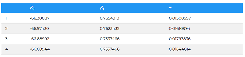
After such sampling, we achieve the sampled data of θ=(β0;β1;τ) such as this

“Cool stuff, so what?”

Now we have 10,000 iterations of the parameter space θ, remember that by equation (1):

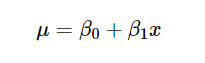
This means that if we substitute x=168cm to each of the iteration, we will find 10,000 values of weight and thus, the distribution of weights given that the height is 168cm.

We are interested in the percentile of my weight, conditional on my height. What we can do is to find the distribution of the percentile of my weight conditional on my height.

Now, what this plot tells us is that my weight (given the 168cm of height) most likely lies around the 0.3 lower percentile of the simulated Vietnamese population.

For example, we can find the percentile that my weight is in the first 40 percentile or less

So there is overwhelming evidence that conditional on my height of 168cm, my weight 58kg would leave me at the lower percentile of the Vietnamese population. Maybe it’s really about time to hit the gym and gain some weights. After all, if you cannot trust some well done Bayesian statistics result, what else can you trust?

I have included in the data source a dataset that that contains the height and weight of 8169 male and female youth in America (National Longitudinal survey 19972), could you conduct the same analysis and see where you stand?

If you enjoy this article, you may also enjoy my other article about interesting statistical facts and rules of thumbs

For other deep dive analyses:

The entire R script for this article can be found at my Github page.

Note: I would like to give a shoutout to Professor Joseph Chang (Yale University) and his class S&DS238: (Bayesian) Probability and Statistics. I took the class almost accidentally and it has easily been one of the most influential classes I have taken (talking about a Political Science major now becoming a Data Scientist)

Data Source: Vuong Q. H.. Open Science Framework. 2017 https://doi.org/10.17605/OSF.IO/AFZ2W