How a 60% Correct AI Model Guides You to Trade with a 90% Success Rate

This is not clickbait. The intuition comes from an MIT course — 15.401 Finance Theory taught by Professor Andrew Lo. Here I used two numbers 60% and 90% as an example. Theoretically, the first number can be any number above 50% and the second number can be any number greater than the first number but less than 100%. Let me explain how that can be achieved mathematically from a financial perspective.

Theoretical Foundation

First of all, let’s justify the meaning of the first number — 60%. I hope you won’t dismiss an AI model with a 60% correct rate. In fact, a 60% correct AI model in predicting the financial market is super good if you believe it really exists. It would be worth a tremendous amount of money if you think about its application in autonomous trading by the big money. We must distinguish this percentage from the performance of other AI models predicting the outcomes of physical laws, which can easily achieve over 99% accuracy. However, whenever you identify a pattern such as a sine curve in the financial market and start to utilize it, the pattern disappears because the market is so competitive (efficient) and other traders have already taken advantage of the arbitrage ahead of you. This contrasts with the patterns governed by the physical laws because the gravitational constant does not change in Newtonian physics and a body in free fall can be accurately predicted in its path and velocity at any time. On the other hand, we set the lower bound of the model correctness to 50%, because if we are certain about a model’s correctness of less than 50%, we just trade the opposite to what the model suggests to gain an advantage.

After we agree that a model with a 60% success rate is actually good to start with, let’s explore how we can maximize its potential in trading. Imagine a scenario in which you are watching two stocks at the same time: Stock A and Stock B. You have $50,000 in cash and wait to trade based on the outputs of the AI model that you have trained up to a success rate of 60%.

Suppose the model’s predictions are as follows:

· Stock A: target increase: 2%, stop-loss: 2%

· Stock B: target increase: 1%, stop-loss: 1%

Well, I know this output does not look promising to many traders, because we all want a target/stop ratio of greater than 1 to actually entice us into a trade. I totally understand. But in this hypothetical demo, I don’t want to introduce any additional advantages of the model other than the 60% correctness as the only edge.

Knowing my model is 60% correct, I may just buy stock A with all my buying power as my Option 1 and the expected profit of this trade is $50,000 x 2% x 0.6 (if my model is right) — $50,000 x 2% x 0.4 (if my model is wrong) = $200.

I could also do Option 2: split my money and buy $25,000 in Stock A and $25,000 in Stock B. By doing so, I can hedge some risk by diversifying the portfolio. Now let’s look at the expected value of this set of trades:

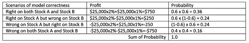
With the table listing all profits and their probabilities, we can compute the expected profit of this set of trades as follows:

$750 x 0.36 + $250 x 0.24 — $250 x 0.24 — $750 x 0.16 = $150

Since we traders are only interested in the first two scenarios with positive profit, which are considered a success, the probability of achieving success is 0.36 + 0.24 = 0.60. This success probability has not yet beaten the model’s correctness rate of 60%, except that the expected profit of the trading activities is reduced from $200 to $150.

Well, what about we redefine success as not having a big loss day? Considering that it is quite normal to have some drawdowns for active traders, as long as we keep our loss small, we will be fine. So, with a new definition of success as not having the worst scenario of losing $750, which has a probability of 0.16, the success probability is computed as 1–0.16=0.84=84%!

If the success redefinition is not acceptable for you and you want the vanilla version of positive profit as success, no hurry. Here comes the magic.

Let’s introduce one more stock to trade and the model’s prediction on that stock is as follows:

· Stock C: target increase: 0.5%, stop-loss: 0.5%

I may still split my money equally and buy $16,667 in Stock A, $16,667 in Stock B, and $16,666 in Stock C. Now let’s compute the expected profit of this set of trades:

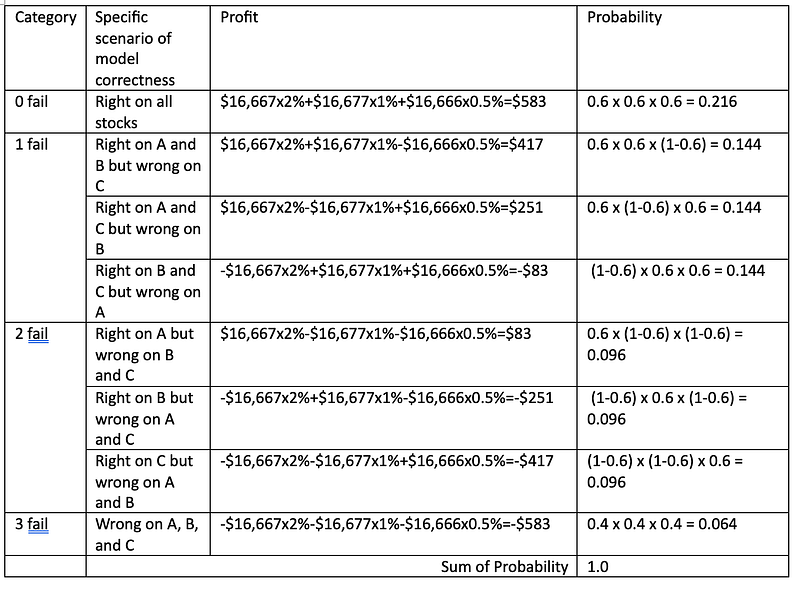
With the table listing all specific scenarios of profits and their probabilities, we can compute the expected profit of this set of trades as follows:

$583 x 0.216 + $417 x 0.144 + $251 x 0.144 -$83 x 0.144 + $83 x 0.096 — $251 x 0.096 — $417 x 0.096 — $583 x 0.061 = $117

We can condense the table by summing up the probability in each category as follows:

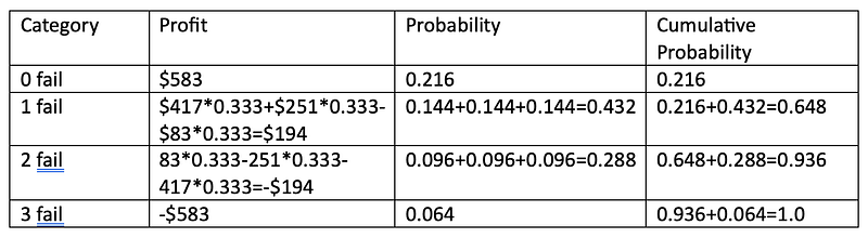
Note that in the profit column, the value of 0.333 is the normalized probability of each specific scenario within the “1 fail” and “2 fail” categories because there are three specific scenarios in each category and each specific scenario in that category has the same probability: 1/3 = 0.333

Suppose we are only interested in the categories with positive profit. Therefore, we only accept “0 fail” and “1 fail” as success. I hope you have noticed that the amazing thing has happened in the column of cumulative probability! The probability of achieving this success is 0.648! This beats the model’s correctness rate of 0.6!

Furthermore, if you are okay with a small loss of $194 by accepting the “2 fail” category, you can achieve a success probability of 0.936!

What happened? It looks like I did not do anything but some simple high school mathematics. MIT Professor Andrew Lo explained an example similar to this but on the topic of fixed-income securities. What he did in his 15.401 class (See his YouTube Video of this lecture at Minute 35:13 here https://www.youtube.com/watch?v=ZWKnK9LIETA) was that he re-allocated the values of two securities by creating senior and junior tranches, while what I did in this demo was I re-allocated the values of trades by creating two definitions of success:

· The positive-profit success can allow 1 failure out of 3 predictions with a probability of 64.8%.

· The no-big-loss success can allow 2 failures out of 3 predictions with a probability of 93.6%.

How can this be used to guide trading?

If you are a discretionary trader, such computations, which can be done automatically with the code to follow, can inform you of your probability of success. It can substantially improve your trading psychology in a high-stress environment. Suppose you know the probability of a trade is 93.6% for not having a big loss and a small loss is what you can accept, would you still be scared of getting into a trade when every setup seems okay?

If you are an algorithmic trader, such computations can be incorporated into the trading decisions to empower your algorithm further.

Code Implementation

Now let’s implement such computations in Python. Here we use Pandas, re, and the combinations function of the itertools library.

import pandas as pd
import re
from itertools import combinations

Then we define the stocks list, their probability list, their percentage change list, their price list (this is used to compute and show the target and stop levels so that we or the algorithm can clearly see such levels), the cash amount, and allocation of the cash to each stock. You can tweak these numbers and add stocks if you wish.

tickers_list = ['A','B','C']
 
probs_list = [0.6,0.6,0.6]
probs_di = dict(zip(tickers_list,probs_list))

perc_list = [2,1,0.5] # assume up and down risks are the same
perc_di = dict(zip(tickers_list,perc_list))

prices_list = [100,250,500]
prices_di = dict(zip(tickers_list,prices_list))

cash = 50_000
equity_list = [16_667,16_667,16_666]
equity_di = dict(zip(tickers_list,equity_list))

With such an allocation of cash, we can compute the expected profit of this trade.

expected_pnl = 0
for ticker in tickers_list:
    expected_pnl += equity_di[ticker]*perc_di[ticker]/100*(probs_di[ticker]-(1-probs_di[ticker]))
print(expected_pnl)

def gen_action_fail_dfs(tickers_list,probs_di,perc_di,prices_di,equity_di):
    scenarios = [f'{i}fail' for i in range(len(tickers_list)+1)]
    scenario_probs = {}
    scenario_pnl = {}
    friction = 0.0 # Feel free to change this number such as 2 cents/share frictions
    for scenario in scenarios:
        fail_num = [int(s) for s in re.findall(r'\d+',scenario)][0]
        if fail_num == 0:
            prob = 1
            earn = 0
            for ticker in tickers_list:
                prob *= probs_di[ticker]
                earn += (equity_di[ticker]*perc_di[ticker]/100-equity_di[ticker]/prices_di[ticker]*friction) 
            scenario_probs[scenario] = prob
            scenario_pnl[scenario] = earn
        elif fail_num == len(tickers_list):
            prob = 1
            earn = 0
            for ticker in tickers_list:
                prob *= (1-probs_di[ticker])
                earn -= (equity_di[ticker]*perc_di[ticker]/100-equity_di[ticker]/prices_di[ticker]*friction)
            scenario_probs[scenario] = prob
            scenario_pnl[scenario] = earn        
        else:
            failed_tickers_li = list(combinations(tickers_list,fail_num))
            prob_li = []
            earn_li = []
            for failed_tickers in failed_tickers_li:
                won_tickers = []
                [won_tickers.append(x) for x in tickers_list if x not in failed_tickers]
                prob = 1
                earn = 0
                for ticker in failed_tickers:
                    prob *= (1-probs_di[ticker])
                    earn -= (equity_di[ticker]*perc_di[ticker]/100-equity_di[ticker]/prices_di[ticker]*friction)
                for ticker in won_tickers:
                    prob *= probs_di[ticker]
                    earn += (equity_di[ticker]*perc_di[ticker]/100-equity_di[ticker]/prices_di[ticker]*friction)
                prob_li.append(prob)
                earn_li.append(earn)
            scenario_probs[scenario] = sum(prob_li)
            norm_prob_li = [x/sum(prob_li) for x in prob_li]
            scenario_pnl[scenario] = sum([a*b for a,b in zip(norm_prob_li,earn_li)])

    action_df = pd.DataFrame(columns=['action','target','stop','prob','perc','worth'],index=tickers_list)
    for ind in action_df.index:
        action_df.loc[ind,['action','target','stop','prob','perc','worth']] = equity_di[ind],prices_di[ind]*(1+perc_di[ind]/100),\
            prices_di[ind]*(1-perc_di[ind]/100),probs_di[ind],perc_di[ind],equity_di[ind]*perc_di[ind]/100*(2*probs_di[ind]-1)-equity_di[ticker]/prices_di[ticker]*friction

    fail_df = pd.DataFrame(columns=['pnl','prob','cum_prob'],index=scenarios)
    for ind in fail_df.index:
        fail_df.loc[ind,['pnl','prob']] = scenario_pnl[ind],scenario_probs[ind]
    fail_df['cum_prob'] = fail_df['prob'].cumsum()
    return action_df,fail_df

def gen_tradable_tickers_di(tickers_list,probs_di,perc_di,prices_di):
    tradable_tickers_di = {}
    friction = 0.0
    min_earn = 0.10 # minimun earn per share
    for ticker in tickers_list:
        expectation = perc_di[ticker]*(2*probs_di[ticker]-1)/100*prices_di[ticker]-friction-min_earn
        if expectation>0:
            tradable_tickers_di[ticker] = expectation
    {k: v for k, v in sorted(tradable_tickers_di.items(), key=lambda item: item[1])}
    return tradable_tickers_di


tradable_tickers_di = gen_tradable_tickers_di(tickers_list,probs_di,perc_di,prices_di)
tradable_tickers_list = list(tradable_tickers_di.keys())

action_df,fail_df = gen_action_fail_dfs(tradable_tickers_list,probs_di,perc_di,prices_di,equity_di)
print(action_df)
print(fail_df)

Then, we reproduce the algorithm as demonstrated in the manual computations shown in the previous tables to generate a clear output as follows:

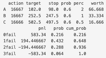
This is the same as the result of the manual computations.

In fact, the above code is more capable than this. You can define the friction and minimum earning per share to filter out the stocks that do not have a good profit potential from your tickers list.

Implications and Concluding Remarks

We have learned in the article that a 60% correct model can easily give us a no-big-loss success probability of over 90%. By introducing more stocks, we have noted the positive-profit success probability can beat the vanilla benchmark of 60% correctness probability of the model.

Although not shown in this article, I have detailed in Chapter 4 Diversified Trading of my book Day Trade with AI with code that (1) by optimizing the allocation of cash in each stock, we can improve the expected profit at the same probability; (2) by generating the model outputs with target/stop ratios of greater than 1, the expected profit can be improved further; and (3) is it possible to generate a model with a higher correctness rate. So, stay tuned and sign up for the mail list when the book becomes available.

Disclaimer:

I do not make any guarantee or other promise as to any results that are contained within this article. You should never make any investment decision without first consulting with your financial advisor and conducting your own research and due diligence. To the maximum extent permitted by law, I disclaim any implied warranties of merchantability and liability in the event any information contained in this article proves to be inaccurate, incomplete, or unreliable or results in any investment or other losses.

I hope you enjoy reading the article. I periodically publish articles of original content on the applications of machine learning and deep learning in the realms of quantitative trading, finance, and engineering. I’m also writing my book Day Trade with AI, which is to be released soon. If you finish reading here and would like to see more of my writings, please follow me on Medium (https://shunyutang.medium.com/), Twitter (https://twitter.com/shunyutang), or Linkedin (https://www.linkedin.com/in/shunyu-tang-31a01a271/).

To support me, you can buy me a coffee by clicking here. I drink a lot of coffee while writing!