Horseshoe priors

Summary

The web content discusses the use of Horseshoe priors as an advanced regularization technique in Bayesian linear regression, which is particularly effective for models with a large number of features.

Abstract

The article delves into the concept of regularization in machine learning, emphasizing the limitations of traditional L1 and L2 regularization methods. It highlights the Horseshoe prior as a superior alternative that addresses the shortcomings of Gaussian (L2) and Lasso (L1) regularization by combining the benefits of both. The Horseshoe prior is shown to be particularly useful in scenarios with a high dimensional feature space, as it can effectively shrink coefficients towards zero while maintaining a balance between model variance and bias. The approach is grounded in Bayesian statistics, where the Horseshoe prior is defined using a half-Cauchy distribution, which has a fat tail and places a non-zero probability mass at zero. This allows for sparsity in the model coefficients, aiding in feature selection without significantly compromising accuracy. The article references the work of Carvalho et al., who introduced the Horseshoe prior and demonstrated its effectiveness through various synthetic data sets.

Opinions

The author expresses that traditional L2 regularization, while useful, does not set parameters to zero and can be problematic with millions of features.
L1 regularization, which can set parameters to zero and thus perform feature selection, is criticized for introducing a bias that reduces accuracy.
The author favors the Horseshoe prior over L1 and L2 regularization because it places a probability mass on zero and has fat tails, which helps reduce both variance and bias.
The article suggests that the Horseshoe prior is a significant improvement in Bayesian linear regression regularization methods, despite the need for hyperparameter tuning due to the No Free Lunch Theorem.
The author believes that the Horseshoe prior has become a standard method for regularization in Bayesian linear regression, as evidenced by its widespread use and further improvements since its introduction.

There are more regularization options than L1 and L2.

Regularization is a fascinating topic, that puzzles me for a long time. First introduced in a machine learning course as a given, it always raised a question why it works. Then I started uncover a connection of regularization to the statistical properties of the underlying model.

Indeed, if we consider linear regression model, it is easy to show, that L2 regularization is equivalent to adding Gaussian noise to the input. In fact, the latter is preferred if we consider feature interactions (or we have to use a non-trivial Tikhonov Matrix, e.g. not proportional to the unit matrix). From the Bayesian perspective, L2 regularization is equivalent to using a Gaussian prior in our model, as explained here. Starting from the Bayesian Linear Regression model, by taking maximum posterior you will receive the L2 regularization term. In general, Normal prior makes the model easy, because Normal distribution is a conjugate prior to the Normal distribution, and this makes the posterior distribution also Normal! If you pick a different prior distribution, then you posterior distribution will be more complex.

The problem with the Gaussian prior and L2 regularization is that it does not set the parameters to zero, but just reduces them. This is especially problematic when we have many features, the situation I had to deal with about 6 months ago, when after all feature processing I had more than 1 million features. In this case we want to use a different kind of regularization, the L1 or Lasso regularization. Instead of adding a penalty of parameter sum of squares, it penalizes based on the sum of the absolute values of parameters. The regularized model sets many parameters to zero, in effect doing for us the task of feature selection. Unfortunately everybody who used it can confirm, that it reduces accuracy rather significantly, because it introduces a bias.

In Bayesian terms, L1 regularization is equivalent to double-exponential prior:

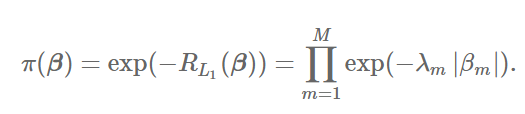
Here and further I follow this case study. The ideal prior distribution will put a probability mass on zero to reduce variance, and have fat tails to reduce bias. Both L1 and L2 fail the test, i.e. both doble-exponential and normal distributions have thin tails, and the probability mass they put at 0 is 0. Please note that in order to put the probability mass > 0 the probability density function must diverge.

A very elegant solution was proposed by Carvalho et al here , here and some other papers. The solution is called Horseshoe prior and is defined like this:

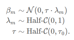
Let me help you decipher this for you. If you remember, L2 regularization is equivalent to having a Normal prior, that is a Normal distribution with mean 0 and the variance that is a hyperparameter that we must tune. (The variance is inverse of the L2 regularization constant λ). In a true Bayesian spirit, we want to define a prior distribution on λ and then marginalize it out. In this approach it is proposed to use a half-Cauchy distribution as a prior distribution. It has been proven that it puts non-zero probability mass at 0, and also has a fat tail. The name “horseshoe” came from the shape of the distribution if we re-parametrize it using this transformation using shrinkage weight k:

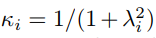
In this case the distribution support changes to [0,1], and when plotted compared to other prior distribution candidates:

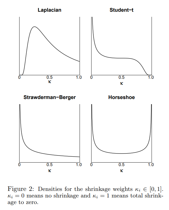
we can see that Horseshoe prior satisfies both of our conditions.

Conclusion

In the papers mentioned above the method was tested in a variety of synthetic data sets, and since then it became one of the standard of Bayesian linear regression regularization methods. It has been improved since then multiple times and tailored for other situations. Of course, due to the Free Lunch Theorem, it is not possible to marginalize out all hyperparameters, so much of the discussion is devoted to tuning the algorithm or overcoming some of its shortcomings.

References

Carvalho, C. M., Polson, N. G. and Scott, J. G. (2009). Handling sparsity via the horseshoe. In Proceedings of the 12th International Conference on Artificial Intelligence and Statistics (D. van Dyk and M. Welling, eds.). Proceedings of Machine Learning Research 5 73–80. PMLR.

Carvalho, C. M., Polson, N. G. and Scott, J. G. (2010). The horseshoe estimator for sparse signals. Biometrika 97 465–480.