Hierarchical Clustering

Hierarchical clustering is a family of clustering algorithms that build a hierarchy of clusters, allowing users to understand the data structure at various granularity levels.

There are two types of hierarchical clustering algorithms:

1. Agglomerative clustering (bottom-up approach) starts with each data point as a separate cluster, and in each successive step merges the two clusters that are closest to each other. This process continues until all data points are in a single cluster. See [1] for a survey of hierarchical agglomerative clustering algorithms.
2. Divisive clustering (top-down approach) starts with all data points in one cluster, and iteratively splits the most heterogenous cluster into two clusters. This process continues until each data point becomes its own cluster.

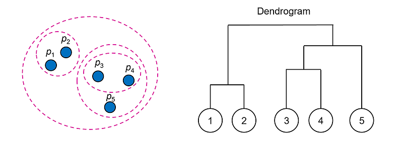
The results of hierarchical clustering are usually presented in a dendrogram. A dendrogram is a tree-like structure that shows the sequence in which clusters were merged (or split) and the distance at which each merge (or split) took place. It is useful for understanding the structure of the data and for determining the desired number of clusters in the final output.

This article explores the various hierarchical clustering algorithms and shows how they can be applied to different types of datasets, highlighting their strengths and weaknesses in various scenarios.

Distance Matrix

The main data structure used by hierarchical clustering algorithms, which allows them to keep track of distances between clusters, is the distance matrix.

Formally, if the dataset has n data points {x₁, …, xₙ}, a distance matrix D is an n × n matrix, where Dᵢⱼ is the distance between points xᵢ and xⱼ. By definition, the distance matrix is symmetric and its diagonal entries are all zeros.

Linkage Methods

In order to decide which clusters to combine (or split), we need a measure of distance between two sets of points (clusters).

A linkage method (or criterion) specifies how distances between clusters are calculated. Commonly used linkage methods include:

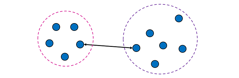
1. Single linkage (MIN) defines the distance between two clusters as the minimum distance between any point in the first cluster and any point in the second cluster.

Pros:

• Can capture clusters of non-elliptical shapes, such as elongated clusters or clusters with more complex geometries.
• Supports various distance metrics.

Cons:

• Sensitive to noise and outliers.
• Prone to the “chaining” effect, where clusters that are actually separate can be connected by a series of intermediate points that act as bridges.

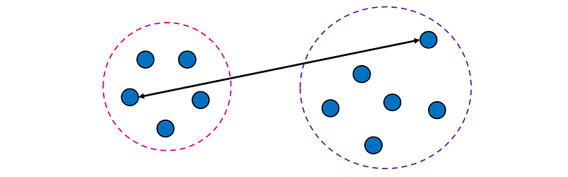
2. Complete linkage (MAX) defines the distance between two clusters as the maximum distance between any point in the first cluster and any point in the second cluster.

Pros:

• Less susceptible to noise and outliers.
• Supports various distance metrics.

Cons:

• Tends to break large clusters.
• Struggles to capture clusters of non-elliptical shape.

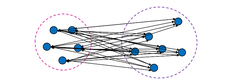
3. Average linkage defines the distance between two clusters as the average distance between each pair of points from the two clusters.

Pros:

• Provides a balance between single and complete linkage.
• Less sensitive to noise and outliers as compared to single linkage.

Cons:

• Biased towards globular clusters.

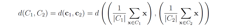
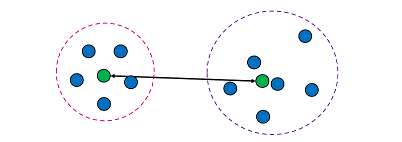
4. Centroid linkage defines the distance between two clusters as the distance between their centroids (or means).

Pros:

• Intuitive, as it considers the central tendency of the clusters.
• Less sensitive to noise and outliers as compared to single linkage.

Cons:

• Less suitable for capturing non-elliptical clusters.
• Can suffer from the “inversion phenomenon”, where merging two clusters decreases their distance to other clusters.
• Supports only the Euclidean distance metric.

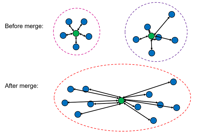
5. Ward’s method [2] defines the distance between two clusters as the increase in the within-cluster sum of squared distances (WCSS) when the two clusters are merged.

where c₁ is the centroid of cluster C₁, c₂ is the centroid of cluster C₂, and c₁,₂ is the centroid of the merged cluster.

A simpler way to write this distance is:

Pros:

• Tends to produce compact and equally-sized clusters (similar to k-means).
• Less sensitive to noise and outliers as compared to single linkage.

Cons:

• Assumes that the clusters have approximately the same size.
• Less suitable for capturing non-elliptical clusters.
• Supports only the Euclidean distance metric.

The Agglomerative Clustering Algorithm

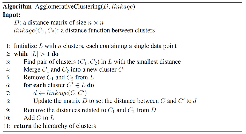
We are now ready to present the agglomerative clustering algorithm. The algorithm gets a distance matrix D and a linkage criterion, and performs the following steps:

1. Initialization: Start with each data point as its own cluster.
2. Iteratively merge the closest clusters until only one cluster is left by following these steps: (a) Find the closest pair of clusters C₁ and C₂ based on the linkage criterion. (b) Merge C₁ and C₂ into a new cluster C. (c) Update the distance matrix by merging the rows and columns of C₁ and C₂, and computing for each cluster C’ the distance between C’ and the new cluster C using the linkage function.

3. Return a hierarchical representation of the clusters.

A pseudocode of the algorithm is shown below:

To obtain a flat clustering structure (similar to the clustering obtain from partition-based methods), one can cut the resulting cluster tree at a specific height. Some implementations of the algorithm allow users to specify a desired number of clusters, and then the algorithm stops once this number is reached.

Time Complexity

In the naive implementation of agglomerative clustering, at each step, the algorithm must search through all pairs of clusters to find the pair with minimum distance to merge. This requires O(n²) comparisons, where n is the number of data points. Since there are n such steps (as we merge two clusters in each step until only one cluster remains), the total time complexity is O(n³). By using a priority queue to store the distances between the clusters, the time complexity can be reduced to O(n² log n).

For specific linkage criteria, optimized algorithms have been developed that can further reduce the time complexity:

• The SLINK algorithm [2] for single linkage clustering has a time complexity of O(n²).
• The CLINK algorithm [2] for complete linkage clustering also operates in O(n²).

All algorithms use O(n²) memory required for storing the distance matrix.

Despite these optimizations, agglomerative clustering is still computational expensive for large datasets as compared to other clustering algorithms like k-means.

Numerical Example

Assume that we have the following dataset with 10 two-dimensional points:

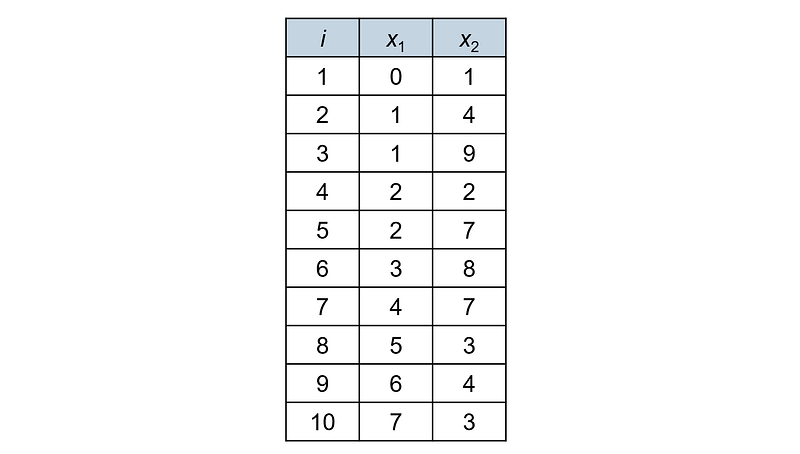
We would like to cluster the data points using hierarchical agglomerative clustering with single linkage and Euclidean distance.

The first step is to compute the distance matrix. To simplify the computations, we will use the squared Euclidean distance instead of the standard Euclidean distance. This change will not impact the clustering outcomes. Since the distance matrix is symmetric, we only need to compute half of it (either the upper triangular half or the lower triangular half).

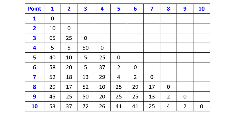
The minimum distance is 2, and there are four pairs of clusters with this distance: (p₅, p₆), (p₆, p₇), (p₈, p₉) and (p₉, p₁₀). Let’s arbitrarily choose the pair (p₅, p₆) and merge them into one cluster. We also update the distance matrix by merging rows 5, 6 and columns 5, 6, and recalculating the distances between the new cluster and all the other data points. Since we are using single linkage, the distance between the new cluster and a point p is equal to the minimum between dist(p₅, p) and dist(p₆, p). For example, the distance between the new cluster and p₁ is min(dist(p₅, p₁), dist(p₆, p₁)) = min(40, 58) = 40.

The updated distance matrix is:

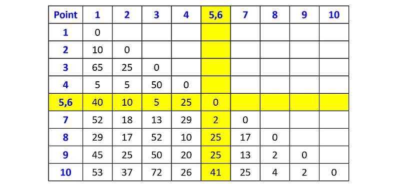
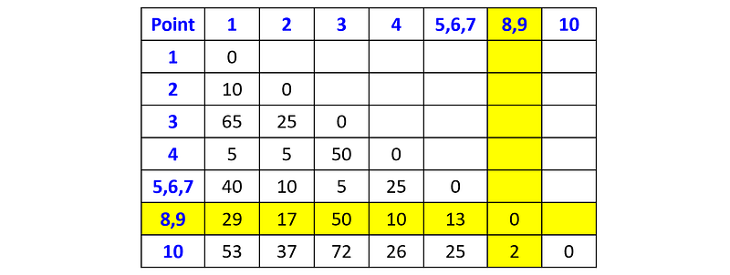
We can now choose either to merge the cluster {p₅, p₆} with point p₇, or to merge one of the pairs (p₈, p₉) or (p₉, p₁₀). Let’s arbitrarily choose the former. In this case, we update the distance matrix by merging the row (5,6) with row 7, and column (5,6) with column 7, and then recompute the distances between the merged cluster (p₅, p₆, p₇) and the other data points:

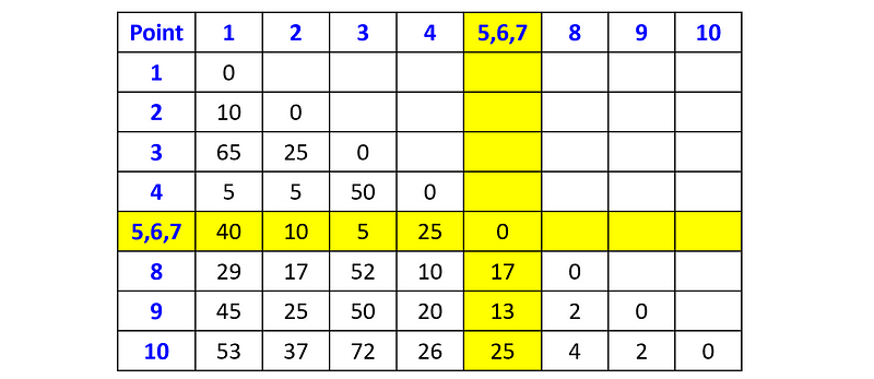
Next, we merge points p₈ and p₉:

And then we merge the cluster {p₈, p₉} with the point p₁₀:

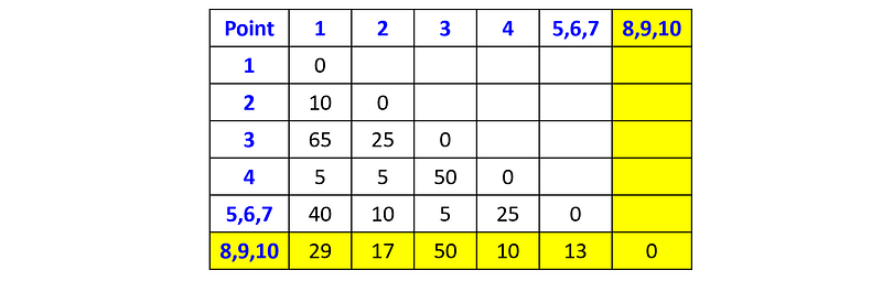
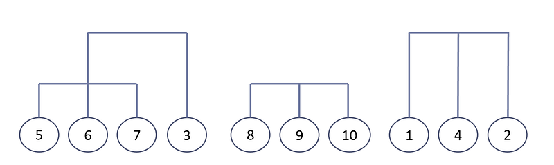
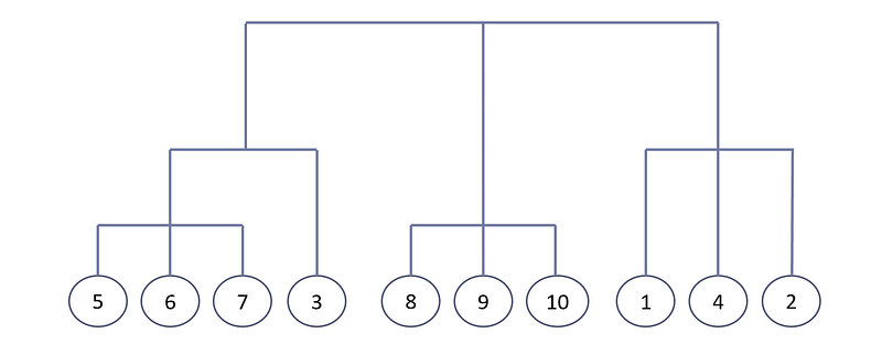
We have finished merging all the clusters with distance 2 between each other. At this point, our dendrogram looks as follows:

The next minimum distance in the matrix is 5. There are three pairs of clusters with this distance: ({p₁}, {p₄}), ({p₂}, {p₄}), and ({p₅, p₆, p₇}, {p₃}). Let’s arbitrarily choose to merge the points p₁ and p₄ into a new cluster. The distance matrix after the merge is:

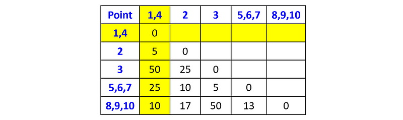
Next, we will merge the cluster {p₁, p₄} with the point p₂:

And now the cluster {p₅, p₆, p₇} with the point p₃:

At this point, the dendrogram looks as follows:

The next minimum distance in the matrix is 10. There are two merges we can choose from at this distance. Let’s start by merging the clusters {p₁, p₄, p₂} and {p₅, p₆, p₇, p₃}:

Finally, we merge the cluster {p₁, p₄, p₂, p₅, p₆, p₇, p₃} with the cluster {p₈, p₉, p₁₀}. The final dendrogram is:

Agglomerative Clustering in SciPy

SciPy is a Python library that provides a collection of mathematical algorithms and convenience functions built on NumPy. Its module scipy.cluster.hierarchy provides functions for hierarchical agglomerative clustering, including functions for generating clusters from distance matrices, calculating statistics on clusters, visualizing clusters with dendrograms, and cutting linkages to generate flat clusters.

The function scipy.cluster.hierarchy.linkage() is the main function for performing agglomerative clustering. It accepts the following parameters:

• y: Can be either a a 2-D array of data points or a condensed 1-D distance matrix (i.e., a flat array containing the upper triangular of the distance matrix).
• method: The linkage method. Can be either 'single' (the default), ‘complete’, 'average', 'weighted', 'centroid', 'median', or 'ward'.
• metric: The distance metric to use (defaults to 'euclidean').

The function returns the clustering encoded as a linkage matrix Z, which has the following structure:

• The first two columns of Z represent the indexes of the clusters that are being merged.
• The third column is the distance between the clusters that were merged.
• The fourth column represents the number of samples in the newly formed cluster.

For example, let’s use this function to perform agglomerative clustering on the toy dataset from the previous section. First, we define the data points:

X = np.array([[0, 1], [1, 4], [1, 9], [2, 2], [2, 7], 
              [3, 8], [4, 7], [5, 3], [6, 4], [7, 3]])

For consistency with our manual computations, we will use the single linkage method and the squared Euclidean distance metric:

from scipy.cluster import hierarchy

Z = hierarchy.linkage(X, method='single', metric='sqeuclidean')
Z

The results of the clustering is:

array([[ 4.,  5.,  2.,  2.],
       [ 6., 10.,  2.,  3.],
       [ 7.,  8.,  2.,  2.],
       [ 9., 12.,  2.,  3.],
       [ 0.,  3.,  5.,  2.],
       [ 1., 14.,  5.,  3.],
       [ 2., 11.,  5.,  4.],
       [15., 16., 10.,  7.],
       [13., 17., 10., 10.]])

These results are consistent with the clustering we have obtained earlier. For example, in the first iteration, points 4 and 5 are merged (the indexes of the points starts from 0) at distance 2 to form a new cluster of two points, whose index is 10. Then, in the second iteration we merge point 6 with cluster 10 (that consists of points 4 and 5) at distance 2 to form a cluster of three points.

To plot the dendrogram, we can call the function scipy.cluster.hierarchy.dendrogram() with the matrix Z:

hierarchy.dendrogram(Z)
plt.xlabel('Data Point Index')
plt.ylabel('Distance')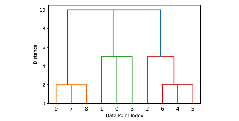

In addition, we can use the function scipy.cluster.hierarchy.fcluster() to obtain flat clusters from the linkage matrix by cutting the dendrogram at a specified level. This function accepts the following parameters:

• Z: The linkage matrix returned from the linkage() function.
• t: The threshold to apply when forming flat clusters.
• criterion: The criterion to use in forming flat clusters. Common criteria include 'distance' for specifying a distance cutoff, and ‘maxclust’ to specify a maximum number of clusters.

The function returns the cluster labels assigned to the data points.

For example, we can obtain a flat clustering from our dendrogram by cutting it at distance of 5:

hierarchy.fcluster(Z, t=5, criterion='distance')

array([2, 2, 3, 2, 3, 3, 3, 1, 1, 1], dtype=int32)

In this case, three clusters are returned: {p₁, p₂, p₄}, {p₃, p₅, p₆, p₇}, and {p₈, p₉, p₁₀}.

Agglomerative Clustering in Scikit-Learn

Scikit-Learn also provides an implementation of agglomerative clustering in the class sklearn.cluster.AgglomerativeClustering. The main differences between the Scikit-Learn and the SciPy implementations are:

1. Scikit-Learn’s AgglomerativeClustering produces a flat clustering based on a predefined number of clusters, rather than generating the full dendrogram. This approach can significantly reduce the runtime needed to find the desired number of clusters. In contrast, the full dendrogram provided by SciPy’s linkage() method allows for more flexibility in post-hoc analysis, such as deciding on the number of clusters after viewing the dendrogram.
2. AgglomerativeClustering is easier to integrate with other Scikit-Learn estimators and utilities due to its compatibility with Scikit-Learn’s API (e.g., it implements the fit() and fit_predict() methods).

The important hyperparameters of the AgglomerativeClustering class are:

• n_clusters: The number of clusters to find (defaults to 2).
• linkage: The linkage method to use. Can be 'ward' (the default), 'single', 'complete', or 'average'.
• metric: The distance metric to use. Can be 'euclidean' (the default), 'l1', 'l2', 'manhattan', 'cosine', or 'precomputed'. If the linkage method is 'ward', then only 'euclidean' is accepted.
• distance_threshold: The distance threshold above which clusters will not be merged (defaults to None). If not None, n_clusters must be set to None.

Let’s demonstrate how to use this class to cluster a synthetic dataset. First, we use the make_blobs() function from sklearn.datasets to create a dataset with 500 points chosen randomly from 3 normally-distributed clusters:

from sklearn.datasets import make_blobs

X, y = make_blobs(n_samples=500, centers=3, cluster_std=0.6, random_state=0)

Next, we normalize the dataset to ensure that all the features are measured on the same scale:

from sklearn.preprocessing import StandardScaler

X = StandardScaler().fit_transform(X)

Let’s plot the dataset:

def plot_data(X):
    sns.scatterplot(x=X[:, 0], y=X[:, 1], edgecolor='k', legend=False)
    plt.xlabel('$x_1$')
    plt.ylabel('$x_2$')

plot_data(X)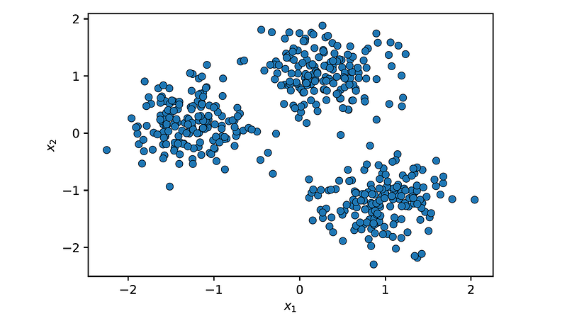

Next, we create an instance of the AgglomerativeClustering class with n_clusters=3 and linkage='single' (the default is 'ward'), and fit it to the dataset:

from sklearn.cluster import AgglomerativeClustering

agg = AgglomerativeClustering(n_clusters=3, linkage='single')
agg.fit(X)

To visualize the clustering results, we will use the following function:

def plot_clusters(X, labels):
    sns.scatterplot(x=X[:, 0], y=X[:, 1], hue=labels, palette='tab10', edgecolor='k', legend=False)
    plt.xlabel('$x_1$')
    plt.ylabel('$x_2$')

plot_clusters(X, agg.labels_)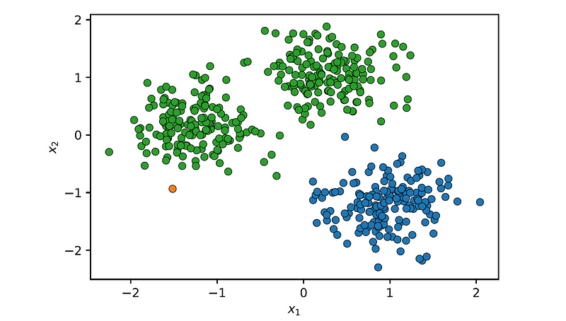

As can be seen, single linkage was unable to identify correctly the clusters. For example, the noise points between the two upper clusters has caused it to merge the two clusters together.

Let’s now try the complete linkage method:

agg = AgglomerativeClustering(n_clusters=3, linkage='complete')
agg.fit(X)

plot_clusters(X, agg.labels_)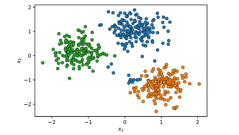

This time, the algorithm has identified the three clusters, but sections of the top-left and right-bottom clusters have been separated, demonstrating the tendency of complete linkage to fragment large clusters.

Finally, let’s use Ward’s method:

agg = AgglomerativeClustering(n_clusters=3, linkage='ward')
agg.fit(X)

plot_clusters(X, agg.labels_)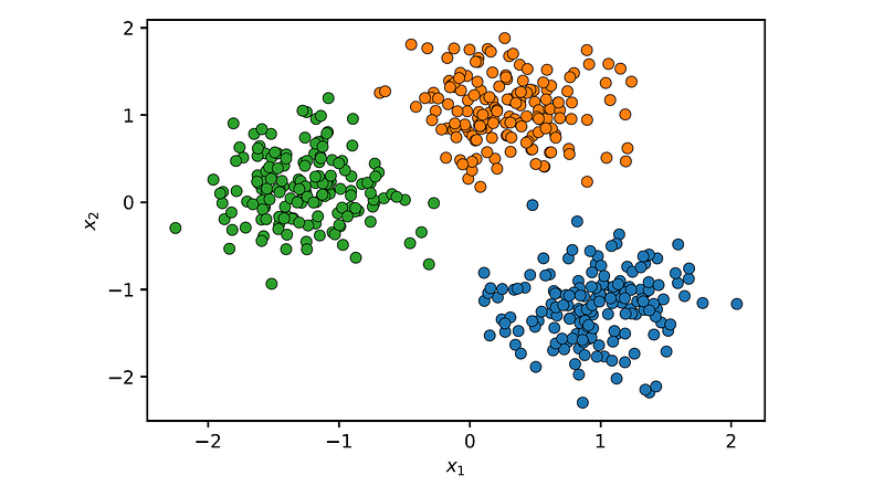

Ward’s method gave the best results on this dataset, since the clusters have spherical shapes and are roughly of equal size. Ward’s method aims to minimize the variance within each cluster, making it particularly suited for datasets with compact and well-defined clusters, as is the case here.

The fastcluster Library

fastcluster is a Python library that provides optimized implementations of hierarchical clustering algorithms, which can work faster than other standard implementations like those in Scipy and Scikit-Learn, especially on large datasets. Its main features are:

• Uses a memory efficient representation of the distance matrix, which can save both computation time and memory when the dataset is large.
• Avoids unnecessary distance recomputations when possible.
• Provides an efficient implementation of the Ward and centroid methods that scales as O(n²logn), whereas a naive implementation requires O(n³).
• Primarily written in C++, which minimizes the overhead associated with Python function calls and data type conversions.

To use fastcluster, you first need to install it using pip:

pip install fastcluster

The main function provided by the library is fastcluster.linkage(), which has exactly the same interface as scipy.cluster.hierarchy.linkage().

For example, let’s compare the execution time of fastcluster with the SciPy implementation on a dataset that consists of 25,000 randomly generated points from three normally distributed clusters:

X, y = make_blobs(n_samples=25000, centers=3, random_state=0)
X = StandardScaler().fit_transform(X)

The time it takes to cluster this dataset using SciPy is:

from scipy.cluster import hierarchy

%timeit Z = hierarchy.linkage(X, method='single')

7.9 s ± 190 ms per loop (mean ± std. dev. of 7 runs, 1 loop each)

And the time it takes to perform the same task with fastcluster is:

import fastcluster

%timeit Z = fastcluster.linkage(X, method='single')

4.83 s ± 54 ms per loop (mean ± std. dev. of 7 runs, 1 loop each)

fastcluster has managed to cut down the runtime by approximately 39%.

Divisive Hierarchical Clustering

Divisive hierarchical clustering is a top-down approach where we start with a single cluster that contains all data points, and iteratively split the clusters into smaller clusters until each cluster contains only one point or until some stopping criterion is met.

Algorithms used for divisive hierarchical clustering include:

1. DIANA (DIvisive ANAlysis) [3] chooses in each step the cluster with the largest diameter (maximum distance between its data points) and splits it into two clusters. The split is done by identifying the point with the maximum average distance to other points in the cluster and then separating data points based on their distance to the identified point.
2. MST-based divisive hierarchical clustering [4] begins by constructing an MST (Minimum Spanning Tree) connecting all the data points such that the total edge weight (sum of distances between connected points) is minimized. It then iteratively splits the dataset into two clusters by removing the longest edge from the MST in each iteration.
3. Bisecting k-means [5] is an iterative variant of k-means, where in each iteration a cluster (usually the one with the highest WCSS or largest size) is split into two clusters using k-means with k = 2. This process continues recursively on the resultant clusters until the target number of clusters is reached. Scikit-Learn provides an implementation of this algorithm in the class sklearn.cluster.BisectingKMeans.

In general, divisive hierarchical clustering methods are less commonly used than agglomerative methods as they tend to be more computationally intensive. This is because for dividing n points into two clusters there are 2ⁿ⁻¹ - 1 possible partitions to be examined, while choosing two out of n clusters to merge requires to consider only n(n -1)/2 possibilities.

Summary

Let’s summarize the pros and cons of hierarchical clustering as compared to other clustering methods.

Pros:

• Outputs a hierarchy of clusters, which provides a more detailed view of the data’s structure compared to partitioning methods such as k-means.
• Can detect non-spherical cluster structures unlike other algorithms such as k-means.
• Supports various linkage methods (e.g., single, complete, average), which can capture various cluster shapes.
• No need to specify the number of clusters in advance. The resultant dendrogram can be cut at various levels to produce different number of clusters.
• Provides a visual representation (dendrogram) that is useful for understanding the data structure and the relationships between clusters.
• The method is deterministic, i.e., it will produce the same clusters in every run.
• Supports various distance metrics.

Cons:

• Computationally intensive, making it less suitable for large datasets.
• Some linkage methods (especially single linkage) are sensitive to outliers, which can cause two significantly separate clusters to merge.
• The choice of linkage method can significantly impact the clustering results.
• Can struggle with detecting clusters with complex geometries (such as clusters located inside each other).
• Deciding where to cut the dendrogram to get a desired number of clusters can be ambiguous and might require domain knowledge.
• The dendrograms are hard to understand and analyze for large datasets.
• There is no clear objective function that the algorithm tries to optimize.

You can find the code examples of this article on my github: https://github.com/roiyeho/medium/tree/main/hierarchical_clustering

References

[1] Müllner, D. (2011). Modern hierarchical, agglomerative clustering algorithms. arXiv preprint arXiv:1109.2378.

[2] Ward Jr, J. H. (1963). Hierarchical grouping to optimize an objective function. Journal of the American statistical association, 58(301), 236–244.

[3] Sibson, R. (1973). SLINK: an optimally efficient algorithm for the single-link cluster method. The computer journal, 16(1), 30–34.

[4] Sneath, P. H., & Sokal, R. R. (1973). Numerical taxonomy. The principles and practice of numerical classification.

[5] Zahn, C. T. (1971). Graph-theoretical methods for detecting and describing gestalt clusters. IEEE Transactions on computers, 100(1), 68–86.

[6] Steinbach, M., Karypis, G., & Kumar, V. (2000). A comparison of document clustering techniques. Department of Computer Science and Egineering, University of Minnesota.